The filters {hp,n(m)}, that model the impulse response be- tween each source sn(k) .... minimize the audiovisual criterion JAV (P(f),t) between the audio spectrum ...
Using audiovisual speech processing to improve the robustness of the separation of convolutive speech mixtures Bertrand Rivet∗† , Laurent Girin∗ , Christian Jutten† and Jean-Luc Schwartz∗ ∗ Speech
Communication Institute (ICP) Grenoble National Polytechnic Institute (INPG) Grenoble, France
Abstract— Looking at the speaker’s face seems useful to better hear a speech signal and extract it from competing sources before identification. In this paper, we present a novel algorithm plugging audiovisual coherence of speech signals, estimated by statistical tools, on audio blind source separation (BSS) algorithms in the difficult case of convolutive mixtures. The algorithm mainly works in the frequency (transform) domain, where the convolutive mixture becomes an additive mixture for each frequency channel. Frequency by frequency separation is made by an audio BSS algorithm, and the audiovisual information is used to solve the standard source permutation problem at the output of the separation stage, for each frequency. The proposed method is shown to be efficient in the case of 2 × 2 convolutive mixtures.
I. I NTRODUCTION
† Image
and Signal Processing Laboratory (LIS) Grenoble National Polytechnic Institute (INPG) Grenoble, France
Section II introduces the BSS problem in convolutive mixtures. Section III explains the audiovisual principle to improve the processing of the permutation ambiguity. Section IV proposes numerical experiments before conclusions and perspectives in section V. II. BSS
OF CONVOLUTIVE MIXTURES
Let us consider the case of a stationary convolutive mixture of N audio sources s(m) = [s1 (m), · · · , sN (m)]T to be separated from P observations x(m) = [x1 (m), · · · , xP (m)]T (T denoting the tranpose): xp (k) =
N ∞ X X
hp,n (m)sn (k − m)
(1)
n=1 m=−∞
Looking at the speaker’s face seems useful to better hear a speech signal and to extract it from competing sources before identification [1]. Schwartz et al. [2] attempted to show that vision may enhance audio speech in noise and therefore provide what they called a “very early” contribution to speech intelligibility, different and complementary to the classical lipreading effect. This suggests to elaborate new speech enhancement or extraction techniques exploiting the audiovisual coherence of speech stimuli. Girin et al. [3] developed a technological implementation of this idea: a first system for automatically enhancing audio speech embedded in white noise by using filters which parameters were partly estimated from the video input. Deligne et al. [4] provided an extension of this work using more powerful implementation tools. Moreover, their system was applied to speech recognition in adverse environment. Girin et al. [5] and then Sodoyer et al. [6] have developed another approach, more general and hopefully more powerful, exploring the link between two signal processing streams that were completely separated: sensor fusion in audiovisual speech processing on the one hand, and blind source separation (BSS) techniques [7], [8], [9] on the other hand. They have proposed to use a statistical model of audiovisual coherence to estimate the separating matrix in the case of a simple additive mixture. The aim of this paper is to present a new principle to solve the permutation problem in the case of convolutive mixtures of speech signals. This paper is organized as follows.
The filters {hp,n (m)}, that model the impulse response between each source sn (k) and the pth sensor, are entries of the mixing filter matrix {H(m)}. The goal of the BSS is to recover the sources by using a dual filtering process: sˆn (k) =
P ∞ X X
gn,p (m)xp (k − m)
(2)
p=1 m=−∞
where {gn,p (m)} are entries of the demixing filter matrix {G(m)}. These filters are usually estimated such that the components of the output signals vector ˆs(m) = [ˆ s1 (m), · · · , sˆN (m)]T are as mutually independent as possible. This problem is generally considered in the dual frequency domain where the short term Fourier transform of (2) and basic algebra manipulation leads to [9]: Sx (m, f ) = Ssˆ(m, f ) = =
H(f )Ss (m, f )H∗ (f ) G(f )Sx (m, f )G ∗ (f )
(3)
G(f )H(f )Ss (m, f )H∗ (f )G ∗ (f )
(4)
where Ss (m, f ), Sx (m, f ) and Ssˆ(m, f ) are the time varying power spectrum density matrices of respectively the sources s(m), the observations x(m) and the output ˆs(m). H(f ) and G(f ) are the frequency response matrices of the mixing and demixing filter matrices (∗ denoting the conjugated transpose). If we assume that the sources are mutually independent (or at least decorrelated) Ss (m, f ) is a diagonal matrix and an
A(t, f1 )
A(t, fL )
···
A(t, f1 ) · · · A(t, fL/2 ) v1 (t)
(a)
Fig. 2.
6000
A(t, fL/2+1 ) · · ·A(t, fL )
v1 (t)
Marginal recursive scheme
0.8
0.7
spectrum (dB)
4000
2000
0
−2000
0.6
0.5
0.4
0.3
−4000
0.2
−6000
v1 (t)
0
0.01
0.02
0.03
0.04
time (s)
0.05
0.06
0.07
0.1
0
1000
2000
frequency (Hz) 3000
(b)
4000
5000
6000
7000
8000
(c)
Fig. 1. Audio and video parameters. Fig. 1(a) shows the two video parameters. Fig. 1(b) displays the temporal windowed signal and fig. 1(c) its spectral local characteristics (obtained by the FFT of the segment in Fig. 1(b)).
efficient separation must lead to a diagonal matrix Ssˆ(m, f ). Thus, a basic criterion for BSS is to adjust the matrix G(f ) so that Ssˆ(m, f ) is as diagonal as possible. This can be done by the joint diagonalization process described in [10], and in the following we used this method. The well-known crucial limitation of the BSS problem is that for each frequency bin, G(f ) can only be provided up to a scale factor and a permutation between the sources, that is: ˆ −1 (f ) G(f ) = P(f )D(f )H
(5)
where P(f ) and D(f ) are arbitrary permutation and diagonal matrices. Pham et al. [11] proposed to reconstruct the complete frequency response {G(f )} by exploiting the continuity between consecutive frequency bins. They select the permutations that assume a smooth reconstruction of the frequency response. III. AUDIOVISUAL
SOLUTION TO THE PERMUTATION PROBLEM
In this paper, we propose a novel approach to the permutation problem exploiting the audiovisual coherence of speech signals. We assume that we want to extract some particular speech source, say s1 (m), from the audio mixtures x(m) and we exploit additional observations, which consist of a video signal v1 (n) extracted from the speaker’s face and synchronous with the acoustic signal s1 . This video signal consists of the trajectory of basic geometric lip shape parameters. It is now classical to consider that the speaker’s lip parameters and the local spectral characteristics of the acoustic signal are related by a complex relationship, and the relationship can be described in statistical terms (see e.g. [12]). Hence, we assume that we can build a statistical model providing the joint probability pAV (S1 (t, f ), v1 (t)) of a video vector v1 (t) = [V1,a (t), V1,b (t)]T containing the lip internal width and height (Fig 1(a)) and an audio vector S1 (t, f ) = [A1 (t, f1 ), · · · , A1 (t, fL )]T containing local spectral characteristics (Fig. 1(c)). These video and audio vectors represent the useful information of a signal frame (Fig. 1). In
this study, this statistical model is chosen to be a mixture of Gaussian kernels. Now, regularizing the permutation problem of frequency ˆ ) that domain BSS consists in searching the permutation P(f ˆ ˆ assumes S1,P(f ˆ ) (t, f ) ≃ S1 (t, f ), where S1,P(f ) (t, f ) are the estimated audio coefficients of the real audio parameters S1 (t, f ), given by (5) from the BSS algorithm of [10] up to the permutation matrix P(f ). To estimate P(f ), we propose to minimize the audiovisual criterion JAV (P(f ), t) between the audio spectrum output on channel 1 and the visual information v1 : ˆ ) = arg min JAV (P(f ), t) P(f (6) P(f )
with h i ˆ 1,P(f ) (t, f ), v1 (t)) . JAV (P(f ), t) = − log pAV (S
(7)
In order to improve the criterion, we introduce the possibility to cumulate the probabilities over time. For this purpose, we assume that the values of audio and visual characteristics at several consecutive time frames are independent from each other and we define an integrated audiovisual criterion by: T JAV (P(f )) =
T −1 X
JAV (P(f ), t)
(8)
t=0
Since there are (N !)L possible permutation matrices if the short term Fourier transform is calculated over L frequencies, it is not possible to attempt an exhaustive research, because of huge computational load. So we first simplify the criterion by using a marginal form (9). Thus, we marginalize the audiovisual probability pAV (S1 (t, f ), v1 (t)) regarding an arbitrary ensemble F of frequencies fj : Z Z F pAV (S1 (t, f ), v1 (t)) = · · · pAV (S1 (t, f ), v1 (t)) dfj,j ∈F / . So the marginal form of the criterion (8) is T JAV
(P(f ), F) =
T −1 X
JAV (P(f ), t, F)
(9)
t=0
with � � JAV (P(f ), t, F) = − log pF AV (S1,P(f ) (t, f ), v1 (t)) .
Exploiting this simplification, we use the following recursive scheme (Fig. 2): 1) first, test the permutation on all audio parameters1 : T T if JAV (J , {1, · · · , L}) < JAV (I, {1, · · · , L}) do the permutation of all coefficients, 1J
is the unitary anti-diagonal matrix, I is the identity matrix.
80
···
A(t, fi )
···
A(t, fL )
A(t, f1 ) · · · A(t, fi ) A(t, fi+1 ) · · · A(t, fL )
v1 (t)
percentage of error
A(t, f1 )
v1 (t)
70
60
50
40
30
20
10
0
−10 0
Fig. 3.
Joint dichotomic scheme
Fig. 4.
number of integration frames
5
10
15
20
25
30
35
Percentage of detection errors versus number of integration frames.
2) then sharpen the estimation of the permutation matrix by testing separately with (9) a permutation on the first half T of the audio parameters set JAV (P(f ), {1, · · · , L/2}) and on the second half of the audio parameters set T JAV (P(f ), {L/2 + 1, · · · , L}), 3) continue with this dichotomic scheme until T JAV (P(f ), {2j − 1, 2j}) for all j = {1, · · · , L/2}. This initialization phase gives a good estimation of the permutation matrix P(f ) but not the best one. So, we refine the estimation by applying the joint criterion (8) also with a dichotomic form (Fig. 3): 1) for all 1 ≤ i ≤ L, test with (8) the permutation matrix P(f ) that only permutes the frequency fi leaving all the other frequencies fj , j 6= i, 2) then, test with the same manner all couples of frequencies {f2i−1 , f2i }, 3) continue with this dichotomic scheme until {f1 , · · · , fL }, 4) loop at stage 1 if necessary. Thus, two stages are required : the first one using a marginal form of the criterion and the second one using the joint criterion. IV. N UMERICAL
EXPERIMENTS
In the following, we consider the case of two sources mixed by 2 × 2 matrices of filters. All mixing filters are artificial finite impulse response filters up to 64 lags with 3 significant echos. They fit a simplified acoustic model of a room impulse response. Since we are dealing with time varying spectrum, the simplest way to calculate the local audio parameters S1 (t, f ) is to subdivide the temporal signal into consecutive blocks and to estimate the spectrum as if the data inside each block come from stationary processes. Moreover, we need synchronous video parameters v1 (t) and local audio parameters S1 (t, f ). Since the video channel is sampled at 50Hz, we choose the length of the temporal block equal to 20ms and the audio signals are sampled at 16kHz. Moreover, in this study we choose a limited number of audio parameters so we subdivide the spectrum into 32 consecutive bands of 250Hz and we calculate the energy of the signal in these bands. Furthermore, the joint statistical model of the audiovisual information consists in a mixture of 16 Gaussian kernels estimated during a training phase using the EM algorithm [13].
percentage of error
100
80
60
40
20
0
−10
−8
Fig. 5.
−6
−4
SNR (dB)
−2
0
2
4
6
8
10
Percentage of detection error versus SNR.
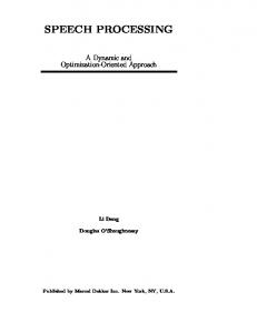
In the following, we present the results of our audiovisual based permutation algorithm. For each experimental condition, the simulation is repeated over 40 different speech sentences. Fig. 4 shows the percentage of detection error2 versus the number of integration frames: the solid line is the mean and the error bars are the standard deviations. This stresses the importance of frames integration for the criteria (8) and (9). Indeed, if the number of frames is too small the number of errors significantly increases while the computation time decreases. Meanwhile, if the number of frames increases, the number of errors decreases towards zero while the computation time increases. So choosing around 20 frames of integration seems to be a good trade-off between computation time and detection error. Fig. 5 displays the percentage of permutation errors versus the signal to noise ratio (SNR) SN R1 with 20 integration frames. The definition of the SNR is SN Ri (dB) = 10 log
Psi Pni
(10)
PT where Psi = t=1 |((GH)ii ∗ si )(t)|2 represents the power contribution of the source PTactual P source si in the estimated 2 |((GH) ∗ s )(t)| for i 6= j sˆi , and Pni = ij j t=1 j6=i represents the interfering power contribution of all the other sources. This figure underlines that our criterion is quite robust to a bad estimation of the separation matrix. The symmetrical aspect of the curve appears normal. Indeed, when the SN R becomes lower than 0dB, the noise power becomes larger than the signal power. In the 2 × 2 case, this is equivalent to say that the estimated source sˆ1 (resp. sˆ2 ) looks more like the real source s2 (resp. s1 ). 2 The permutation errors contain both the unsolved permutations (actual permutations undetected by our algorithm) and the wrong permutations (bad decision of the algorithm).
0.1
0.03
0.1
0.1
0.02 0.05
0.05
0.01
0.05
0
0 0
0
−0.05
−0.05
−0.01
−0.05
−0.02 −0.03 −0.04
−0.1
−0.1 0
0.1
0.2
0.3
0.4
0.5
0.6
0.7
0.8
0.9
1
0
0.1
0.2
0.3
0.4
0.5
0.6
0.7
0.8
0.9
1
0
0.1
0.2
0.3
0.4
0.5
0.6
0.7
0.8
0.9
1
−0.15
0.1
0.04
0.05
0.02
0
0
0
−0.05
−0.02
−0.02
0.03 0.02
0.1
0.2
0.3
0.4
0
0.1
0.2
0.3
0.4
0.5
0.6
0.7
0.8
0.9
1
0.5
0.6
0.7
0.8
0.9
1
0.02
0.01 0
0
0.04
−0.01 −0.02 −0.03
−0.04
−0.04 0
0.1
0.2
0.3
0.4
0.5
0.6
time (s)
0.7
0.8
0.9
1
(a) Sources
0
0.1
0.2
0.3
0.4
0.5
0.6
time (s)
0.7
0.8
0.9
1
(b) Estimated sources without permutation cancelation 5
0
0.1
0.2
0.3
0.4
1.5
2
1
1
0.5
0.7
0.8
0.9
1
0.5
4
2
3
0.6
(c) Estimated sources with our algorithm
2.5
4
0.5
time (s)
−0.05
0 0
0.1
0.2
0.3
0.4
0.5
0.6
0.7
0.8
0.9
1
0
100
200
300
4
0
0.5
4
0.4
3
0
(d) Estimated sources with artificial cancelation of interference
0.4
0.05
3 0.3
0.3 2
2 0.2
0.2 1
0
100
200
300
0
2.5
0.5
time (s)
1
0.1
0
2000
4000
6000
8000
0
0
2000
4000
6000
8000
0
0.1 0 0
2000
4000
6000
8000
0
2000
4000
6000
8000
2000
4000
6000
8000
0.5
0.08 0.06
3
0.04 0.02
2
0.4
2
0.4
2
1.5
0.3
1.5
0.3
1.5
1
0.2
1
0.2
1
0.5
0.1
0.5
0.1
0.5
2
0 −0.02
1
−0.04 −0.06 0
0.1
0.2
0.3
0.4
0.5
0.6
time (s)
0.7
0.8
0.9
1
(e) Mixtures
0
0
100
200
frequency (Hz)
300
0
0
100
200
frequency (Hz)
300
(f) Global filter for Fig. 6(b) Fig. 6.
0
2000
4000
6000
frequency (Hz)
8000
0
0 0
2000
4000
6000
frequency (Hz)
(g) Global filter for Fig. 6(c)
8000
0
2000
4000
6000
frequency (Hz)
8000
0
0
frequency (Hz)
(h) Global filter for Fig. 6(d)
Sources, mixtures, estimated sources and global filters.
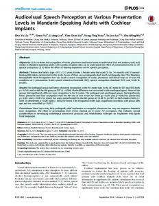
Fig. 6 presents an example of the achieved separation: Fig 6(a) shows the two sources, Fig 6(e) the two mixtures and Fig. 6(b) the two estimated sources given by the BSS algorithm, with a given permutation displayed (Fig. 6(f)) by the spectrum |G(f )H(f )| of the global filter (G ∗ H)(n). Fig. 6(c) (resp. 6(g)) displays the estimated sources (resp. the spectrum of the global filter) after our algorithm. One can see that, for all frequencies f , |(GH)12 (f )| is much smaller than |(GH)11 (f )| and |(GH)21 (f )| is much smaller than |(GH)22 (f )| (care for the axes scale). This first means that our algorithm found all the permutations and also that the two sources are nearly separated. This can be verified with the two last figures 6(d) and 6(h) which show the expected sources if the global filter G(f )H(f ) is effectively diagonal. We obtained this simulated case by forcing to zero the filters (GH)12 (f ) and (GH)21 (f ). V. C ONCLUSIONS
0
AND PERSPECTIVES
The BBS problem of convolutive speech mixtures can be achieved by using a joint diagonalization process in the timefrequency domain [11]. However, this only gives a solution up to a permutation matrix. In this paper, we proposed a new method to overcome this problem exploiting the audiovisual coherence of speech. We showed the importance to cumulate the probabilities on consecutive frames in order to adequately exploit this coherence. Moreover, our algorithm is quite robust regarding the estimation of the separation matrix. As a further steep, we will also extend this method to use directly all the frequency spectrum coefficients instead of a limited number of audio parameters. It is important to note that although the presented results concerned the mixing of two speech sources, our algorithm can be used to extract a
speech signal corrupted by any kind of noisy environment. This point is part of our future works. R EFERENCES [1] K. Grant and P. Seitz, “The use of visible speech cues for improving auditory detection of spoken sentences.” J. Acoust. Soc. Am., vol. 108, pp. 1197–1208, 2000. [2] J.-L. Schwartz, F. Berthommier, and C. Savariaux, “Audio-visual scene analysis; evidence for a ”very-early” integration process in audio-visual speech perception.” in Proc. ICSLP’2002, 2002, pp. 1937–1940. [3] L. Girin, J.-L. Schwartz, and G. Feng, “Audio-visual enhancement of speech in noise,” Journal Accoustical Society of Smerica, vol. 109, no. 6, pp. 3007–3020, june 2001. [4] S. Deligne, G. Potamianos, and C. Neti, “Audio-visual speech enhancement with AVCDCN (AudioVisual Codebook Dependent Cepstral Normalization).” in Proc. ICSLP’2002, 2002, pp. 1449–1452. [5] L. Girin, A. Allard, and J.-L. Schwartz, “Speech signals separation: a new approach exploiting the coherence of audio and visual speech,” in IEEE Int. Workshop on Multimedia Signal Processing (MMSP’2001), Cannes, France, 2001. [6] D. Sodoyer, J.-L. Schwartz, L. Girin, J. Klinkisch, and C. Jutten, “Separation of audio-visual speech sources.” in Eurasip JASP, 2002, pp. 1164–1173. [7] J.-F. Cardoso, “Blind signal separation : statistical principles,” Proceedings of the IEEE, vol. 86, no. 10, pp. 2009–2025, October 1998. [8] C. Jutten and A. Taleb, “Source separation : from dusk till dawn,” in Independant compoment analysis 2000, Helsinki, Finlande, June 2000, pp. 15–26. [9] A. Hyv¨arinen, J. Karhunen, and E. Oja, Independent Component Analysis. New York: Wiley, 2001. [10] D.-T. Pham, “Joint approximate diagonalization of positive definite matrices,” SIAM J. Matrix Anal. And Appl., vol. 22, no. 4, pp. 1136– 1152, 2001. [11] D.-T. Pham, C. Servi`ere, and H. Boumaraf, “Blind separation of convolutive audio mixtures using nonstationary,” in Proceeding of ICA 2003 Conference, Nara, Japan, April 2003. [12] H. Yehia, P. Rubin, and E. Vatikiotis-Bateson, “Quantitative association of vocal-tract and facial behavior.” Speech Communication, vol. 26, pp. 23–43, 1998. [13] A. P. Dempster, N. M. Laird, and D. B. Rubin, “Maximum-likelihood from incomplete data via the em algorithm,” J. Royal Statist. Soc. Ser. B., vol. 39, 1977.