Using Bayesian networks for decision in the simultaneous faults case

Using Bayesian networks for decision in the simultaneous faults case Sylvain Verron, Philippe Weber, Didier Theilliol, Teodor Tiplica, Abdessamad Kobi, Christophe Aubrun

To cite this version: Sylvain Verron, Philippe Weber, Didier Theilliol, Teodor Tiplica, Abdessamad Kobi, et al.. Using Bayesian networks for decision in the simultaneous faults case. Workshop on Advanced Control and Diagnosis (ACD’08), 2008, Coventry, United Kingdom. 2008.

HAL Id: inria-00517096 https://hal.inria.fr/inria-00517096 Submitted on 13 Sep 2010

HAL is a multi-disciplinary open access archive for the deposit and dissemination of scientific research documents, whether they are published or not. The documents may come from teaching and research institutions in France or abroad, or from public or private research centers.

L’archive ouverte pluridisciplinaire HAL, est destin´ee au d´epˆot et `a la diffusion de documents scientifiques de niveau recherche, publi´es ou non, ´emanant des ´etablissements d’enseignement et de recherche fran¸cais ou ´etrangers, des laboratoires publics ou priv´es.

Using Bayesian networks for decision in the simultaneous faults case Sylvain Verron ∗ Philippe Weber ∗∗ Didier Theilliol ∗∗ Teodor Tiplica ∗ Abdessamad Kobi ∗ Christophe Aubrun ∗∗ ∗

LASQUO/ISTIA, 49000 Angers, France (Tel: (33) 241 226 533; email:{sylvain.verron,teodor.tilplica,abdessamad.kobi}@univ-angers.fr). ∗∗ Centre de Recherche en Automatique de Nancy (CRAN), 54506 Vandoeuvre, France (Tel: (33) 383 684 465; e-mail:{philippe.weber,didier.theilliol,christophe.aubrun}@cran.uhpnancy.fr) Abstract: The purpose of this article is to present a new method for process diagnosis with Bayesian network. The interest of this method is to propose a new structure of Bayesian network allowing to diagnose a system with the model-based framework or with the data-driven framework. A particular interest of the proposed approach is the use of continuous nodes in the network in order to evaluate the status of the process. The effectiveness and performances of the method are illustrated on a heating water process corrupted by various faults. 1. INTRODUCTION Nowadays, industrial processes are more and more complex (lots of sensors and actuators). Consequently, an important amount of data can be obtained from a process. A process dealing with many variables can be named multivariate process. But, the monitoring of a multivariate process cannot be reduced to the monitoring of each process variable because the correlations between the variables have to be taken into account. Process monitoring is an essential task. The final goal of the process monitoring is to reduce variability, and so, to improve the quality of the product (Montgomery (1997)). The process monitoring comprises four procedures: fault detection (decide if the process is under normal condition or out-of-control); fault identification (identify the variables implicated in an observed out-of-control status); fault diagnosis (find the root cause of the disturbance); process recovery (return the process to a normal status). Three major kinds of approaches exist for process monitoring (Chiang et al. (2001)): data-driven, model-based and knowledge-based. Theoretically, the best method is the model-based one because this method constructs mathematic models of the process. But, for large systems (lots of inputs, outputs and states), obtaining detailed and reliable models is very difficult. In the knowledge-based category are placed methods based on qualitative models like fault tree, FMECA, expert systems (Venkatasubramanian et al. (2003)). Finally, data-driven methods are techniques based on rigorous statistical development of process data. The purpose of this article is to present a new method for the diagnosis of faults in industrial systems. This method is based on Bayesian networks. The major interest of this method is the diagnosis of the system when multiple faults occurred simultaneously. Moreover, this method is general enough in order to be applicable for model-based fault diagnosis and for data-driven fault diagnosis.

The article is structured in the following manner. In section 2, we introduce the fault diagnosis framework, and briefly detail the model-based fault diagnosis approach, the data-driven fault diagnosis approach, and give some links between these two approaches. The section 3 presents some previous works about the use of Bayesian networks for both approaches of fault diagnosis (model-based and data-driven). In section 4, we propose a new method for fault diagnosis using Bayesian networks, and evaluate it on an heating water process in section 5. Finally, section 6 concludes on interests and limitations of this method, and presents some perspectives of the fault diagnosis with Bayesian networks. 2. FAULT DIAGNOSIS FRAMEWORK 2.1 Model-based fault diagnosis In the model-based fault diagnosis, an analytical model of the process is exploited. For each sample instant, the model gives the normal (fault free) value of each sensors or variables of the system. At this step, residuals are generated. Residuals are defined as the difference between a measurement and the corresponding reference value estimated with the model of the fault-free system (Fig. 1). Inputs

Process

Residuals Generator

Outputs

Residuals r

Fig. 1. Illustration of residuals generator While a single residual is sufficient to detect a fault, a set of residuals is required for fault isolation. Several methods

have been proposed in the literature to generate structured residuals and to perform the fault diagnosis (Isermann and Ball (1996)). One of the most popular methods is the observer-based design (Frank (1990), Patton et al. (2000)). The causal knowledge-based addressed in (Montmain and Gentil (2000)) deals with the complexity of large scale systems. Another way to generate structured residuals is to develop models having an appropriate structure. The structured residuals may be generated by parity equations from the input-output model, or balance equations (chapters 6 and 9, Gertler (1998)). The objective is to decouple the faulty effects from each residual. Each residual is designed so that it is sensitive to different faults or subsets of faults. Once the residuals generated, the fault diagnosis is based on their evaluations. A classical assumption is that the model of the process is defined in such a way that each residual, in the fault-free case, follows a Gaussian distribution. So, statistical hypotheses tests are generally used in order to decide if a residual is significant (fault in the process) or not (no fault in the process): H0 : the residual is not affected by a fault; H1 : the residual is corrupted by a fault. This statistical test implicates two possible errors: α (error of the first kind) giving false alarm rate of the test; and β (error of the second kind) giving the missed detection rate (Basseville and Nikiforov (1997)) of the test. An illustration of the test and the associated errors are given on the Fig. 2.

In the Table 1, a ”1” denotes that a symptom uj is sensitive to a fault (F 1, F 2 or F 3), while a ”0” denotes insensitivity to a fault. This table is called an incidence matrix and can be considered as an a priori knowledge. Each column of the incidence matrix represents a fault signature: the vector [0 1 1]T corresponds to the signature of the faulty element F 1. 2.2 Data-driven fault diagnosis In the data-driven fault diagnosis, the diagnosis procedure can be seen as a classification task (Chiang et al. (2001)). Indeed, today’s processes give many measurements. These measurements can be stored in a database when the process is in fault-free case, but also in the case of identified fault. Assuming that the number of types of fault (classes) and that the belonging class of each observation is in the database (learning sample), the fault diagnosis can be viewed as a supervised classification task whose objective is to class new observations to one of the existing classes Denoeux et al. (1997). For example, given a learning sample of a bivariate system with three different known fault as illustrated in the Fig. 3, we can easily use supervised classification to classify a new faulty observation.

F3

F1

0,45

H1: residual affected

H0: residual not affected by a fault 0,4 0,35

A Pr(x=X)

0,3

F2

0,25 0,2 0,15 0,1

Fig. 3. Bivariate system with three different known faults

0,05

β

α

0 -3

-2,5

-2

-1,5

-1

-0,5

-0

0,5

1

1,5

2

2,5

3

3,5

4

4,5

5

X

Fig. 2. Illustration of the error of the first kind α and error of the second kind β For a given residual, uj represents the status of the residuals (symptoms): uj is equal to ”0” when the residual signal is closer to zero in some sense and equal to ”1” otherwise. Several approaches have been proposed to generate structured residuals and consequently to generate the incidence matrix (Frank (1990)). Let us consider the following example where three different faults (F 1, F 2 and F 3) can be isolated by designing three symptoms u1, u2 and u3 (Table 1).

u1 u2 u3

F1 0 1 1

F2 1 0 0

F3 0 0 1

Table 1. Incidence matrix

Many classifiers have been developed, we can cite FDA (Fisher Discriminant Analysis) (Duda et al. (2001)), SVM (Support Vector Machine) (Vapnik (1995)), kNN (knearest neighborhood) (Cover and Hart (1967)), ANN (Artificial Neural Networks) (Duda et al. (2001)) and Bayesian classifiers (Friedman et al. (1997)). One of the major problem of the classification techniques for the fault diagnosis is the assumption that only one fault can occur simultaneously. This is a problem because, in many situations, multiple faults can occurred at the same time. A possibility to obtain a diagnosis taking into account multiple faults occurrence is to use statistical tests like T 2 control chart (Hotelling (1947)) on each classes of known fault (Verron et al. (2008)). But, for this case, a lot of data is needed. 2.3 Linkings As we have seen in previous sections, data-driven or model-based diagnosis use hypotheses tests in order to decide if a symptom is present in the process. Knowing

the different symptoms of the process, a decision can be made with the help of the incidence matrix. In the datadriven approach, inputs of the statistical tests are directly the variables of the process or computed features from the variables (like principal component analysis (Jackson (1985))). In the case of the model-based fault diagnosis, inputs of the statistical tests are the residuals obtained from the residuals generator. However, in each case, an assumption is made on the data (the residuals or directly the variables). This assumption is that the data follows normal (Gaussian) distribution. So, in the two approaches, statistical tests implicating Gaussian variables is needed. Gaussian variables are continuous variables, but symptoms and decisions are discrete variables. An interesting tool allowing to treat these two kinds of variables is the Bayesian network. Moreover, some approaches for the fault diagnosis using Bayesian networks (model-based and datadriven approaches) have already been developed. A Bayesian Network (BN) (Jensen (1996)) is an acyclic graph where each variable is a node (that can be continuous or discrete). Edges of the graph represent dependences between linked nodes. A formal definition is given here: A Bayesian network is a triplet {G, E, D} where: {G} is a directed acyclic graph, G = (V, A), with V the ensemble of nodes of G, and A the ensemble of edges of G, {E} is a finite probabilistic space (Ω, Z, p), with Ω a nonempty space, Z a collection of subspace of Ω, and p a probability measure on Z with p(Ω) = 1, {D} is an ensemble of random variables associated to the nodes of G and defined on E such as: n Y p(V1 , V2 , . . . , Vn ) = p(Vi |C(Vi )) (1)

u1 u2 u3

In (Weber et al. (2006)), authors propose a Bayesian network in order to model the incidence matrix and the associated decision given the different symptoms of the system. Before to expose this method, we define Bayesian network. The relationship between symptoms and faults are represented by a graph. Obviously a fault can be considered as the cause of the residual deviation. Therefore, some connections can be established from the fault to the symptoms in order to define the relation of causality between fault occurrence and the symptom states. Whereupon, a Bayesian network can define directly an incidence matrix D(n, j). Let us consider two incidence matrices that represent two different cases of possible isolability conditions (Fig. 4). The modelling of the incidence matrices with Bayesian networks is given under the two incidence matrices. The proposed structure is interesting. But, this technique implicates a loss of information (Dougherty et al. (1995)).

F3 0 0 1

u1 u2 u3

F1 0 1 1

F2 1 0 1

F3 1 1 0

F2

F3

F1

F2

F3

u1

u2

u3

u1

u2

u3

Fig. 4. Modelling of incidence matrices with BN Indeed, inputs of the networks are not the residuals (continuous values), but the symptoms (discrete values obtained from the results of statistical tests). 3.2 Data-driven fault diagnosis In (Verron et al. (2007)), authors have demonstrated that a T 2 control chart (Hotelling (1947)) could be modelled with a Bayesian network. For that, two nodes are used: a Gaussian multivariate node X representing the data and a bimodal node F representing the state of the process. The bimodal node F has the following modalities: IC for in control and OC for out-of-control. Assuming that µ and Σ are respectively the mean vector and the variancecovariance matrix of the process, the process can be monitored with the following rule: if P (IC|x) < P (IC) then the process is out-of-control (a fault has occurred in the process). This Bayesian network is represented on the Fig. 5, where the conditional probabilities tables for each node are given. F

F

IC P(IC)

X

F IC OC

with C(Vi ) the ensemble of causes (parents) of Vi in the graph G.

3.1 Model-based fault diagnosis

F2 0 1 0

F1

i=1

3. PREVIOUS WORKS WITH BAYESIAN NETWORKS

F1 1 0 0

OC P(OC)

X X ∼ N (µ, Σ) X ∼ N (µ, c × Σ)

Fig. 5. Control chart with Bayesian network The coefficient c implicated in the modelling of the control chart by Bayesian network (Fig. 5) is the root (different of 1) of the following equation (Verron et al. (2007)): 1−c+

pc ln(c) = 0 LC

(2)

where p is the dimension (number of variables) of the system to monitor, and CL is the control limit of the equivalent T 2 control chart. Very often, CL is equal to χ2α,p , the quantile at the value α of the distribution of the χ2 with p degree of freedom (Montgomery (1997)). So, α allows to tune the false alarm rate of the control chart. 4. THE PROPOSED APPROACH In this section, we propose a new structure of Bayesian network for the fault diagnosis of systems. This new structure is based on the association of the two previous works presented in the last section.

As we have already described, the approach of (Weber et al. (2006)) uses the symptoms (results of hypotheses tests) as observations for the network. But, as the symptoms is discretized (a continuous measure is transformed in ”0” or ”1”), this method loses some information from the process. So, a more interesting technique is to treat the continuous values (values of the residuals) directly in the network. This procedure has two advantages. Firstly, as we have said before, no information is lost. Secondly, the task of hypotheses tests is directly made in the network, and so the evaluation of residuals is transparent. For this approach, we can use the modelling of control chart in a Bayesian network. Indeed, as demonstrated in (Montgomery (1997)), a control chart is a suite of hypotheses tests. The control chart previously presented is a multivariate control chart (taking into account multivariate data). However, the univariate case is simply a specific case of the multivariate control chart. So, the following structure (Fig. 6) is proposed in order to deal directly with the residuals of the analytical model. This is the structure of the right incidence matrix of the Fig. 4.

F1

F2

this data-driven case, continuous variables can have correlations between them. So, in this case, correlations will be represented as edges between the correlated variables. One commonly used data-driven algorithm for this structure learning is called PC (Spirtes et al. (1993)), which uses a series of statistical significance tests of conditional independence. For Gaussian nodes, PC uses the tests of partial correlation with Fisher’s z-transform (Kalisch and Buhlmann (2007)). 5. APPLICATION 5.1 Process description To illustrate our approach, we proposed to consider a simulation example: a heating water process. The process is presented in Fig. 7. Qi Ti

V

T sensor Q0 sensor

F3 R1 P

r1

r2

Q0 T

r3

H sensor

Fig. 6. The proposed structure The Conditional Probabilities Table (CPT) of the two different types of nodes (discrete and continuous) are given in Tables 2 and 3. Fi IC P (IC)

OC P (OC)

Table 2. CPT of the discrete nodes Fk IC IC OC OC

Fk+1 IC OC IC OC

ri 2 ) r3 ∼ N (µri , σri 2 ) r3 ∼ N (µri , cα% × σri 2 ) r3 ∼ N (µri , cα% × σri 2 ) r3 ∼ N (µri , cα% × σri

Table 3. CPT of the continuous nodes In Table 3, µri and σri are respectively the mean and the standard deviation of the residual ri for the free-fault conditions. We also precise that cα% is the coefficient c (equation 2) for a false alarm rate of α percent. Values of cα% for different α are given in Table 4. α cα%

0.1 11.93

0.05 42.57

0.02 218.58

0.01 754.54

0.005 2634.50

H

R2

0.0027 8092.96

Fig. 7. The studied system: a heating water process It is composed of a tank equipped with two heating resistors R1 and R2 . The inputs are the water flow rate Qi , the water temperature Ti and the heater electric power P . The outputs are the water flow rate Q0 and the temperature T which is regulated around an operating point. The temperature of the water Ti is assumed to be constant. The objective of the thermal process is to assure a constant water flow rate with a given temperature. In this analysis only sensor and components failures are considered: level sensor H, output temperature sensor T and output flow rate sensor Q0 . The detailed mathematical model of the simulated system can be found in (Weber et al. (2008)). From model-based fault diagnosis, a classical observer scheme approach is considered. Based on a state space representation of the system around an operating condition where output vector is equal to [H T ]T and input vector [Qi P ]T , structured residual are generated and evaluated in order to detect when H level sensor or T temperature sensor faults occur. Moreover according to the physical equation between output flow rate Q0 and liquid level H, other residual could be established, the fault incidence matrix is defined in Table 5.

Table 4. Values of cα% for different α

An other interesting aspect of the proposed approach is the fact that we can use this model for both: modelbased fault diagnosis, and also data-driven fault diagnosis. Indeed, instead to input the residuals into the network, we can input directly the measurement of the process. But, in

u1 u2 u3

H 0 1 1

Qo 0 0 1

T 1 0 0

Table 5. Incidence matrix of the heating water process

5.2 Construction of the bayesian network

5.3 Results

Based on the incidence matrix of the process (Table 5), the structure of the bayesian network for the diagnosis of the heating water process is constructed (Fig. 8). We precise that in both cases (model-based fault diagnosis and datadriven fault diagnosis) the incidence matrix is the same.

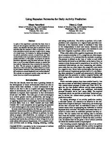
The results of the simulation are given on the following graphs (Fig. 9). These graphs represent the respective a posteriori probabilities of each fault, given the observations (r or x). For a given observation instant and a given fault, if the a posteriori probability of the fault is greater than the a priori probability of the fault (here, fixed to 0.5), then we can say that the fault has occurred in the process.

T

H

Q0

Fault on T 1

r2

r3

Fig. 8. Bayesian network for the fault diagnosis of the heating water process We define the different conditional probabilities tables (CPT) as indicated in Tables 6, 7 and 8. We precise that for each discrete node (the different faults), we have decided to place the a priori probabilities to 0.5. So, it signifies that if an a posteriori probability of a fault is greater than 0.5, then this fault is detected in the process. Concerning the continuous node, we have decided that in the case of a sole conditional fault under the residual, we adopt an α of 2%, but in the case of more faults, we adopt 1% (see Table 8).

H IC IC OC OC

Q0 IC OC IC OC

r3 2 ) r3 ∼ N (µr3 , σr3 2 ) r3 ∼ N (µr3 , c2% × σr3 2 ) r3 ∼ N (µr3 , c2% × σr3 2 ) r3 ∼ N (µr3 , c1% × σr3

Table 8. CPT of the node r3

In the case of the data-driven fault diagnosis, we have exactly the same structure and conditional probabilities tables, except that parameters µri and σri are replaced by µxi and σxi for i = 1, 2, 3. We have simulated the process under the following scenario: • Samples 1 to 9: the system is in a fault-free case. • Samples 10 to 14: a bias on the sensor Q0 is assumed to occur after sample k=9 and to vanish after sample k=14. • Samples 15 to 27: the system is in a fault-free case. • Samples 28 to 40: T and H sensors faults are supposed to occur simultaneously after sample k=27. All the simulations have been made with Matlab/Simulink and the BNT (BayesNet Toolbox) developed by Murphy (Murphy (2001)).

0.2 5

10

15 20 25 Observation instant Fault on H

30

35

40

5

10

15 20 25 Observation instant

30

35

40

30

35

40

0.8 0.6 0.4 0.2

Fault on Qo 1 P(Qo=OC|r or x)

Table 7. CPT of the nodes r1 and r2

0.4

0

Table 6. CPT of the nodes T, H and Q0 r1 or r2 2 ) ri ∼ N (µri , σri 2 ) ri ∼ N (µri , c2% × σri

P(Fault)

1

T, H & Q0 IC OC 0.5 0.5

T or H IC OC

Data-driven

0.6

0

P(H=OC|r or x)

r1

P(T=OC|r or x)

Model-based

0.8

0.8 0.6 0.4 0.2 0

5

10

15 20 25 Observation instant

Fig. 9. Results of the simulation On the Fig. 9, on each graphs, straight lines represents the fixed a priori probabilities of each fault. So, these lines can be named decision limits. The first interesting remark is to view that there are very low variations between the model-based and the data-driven approaches. These variations are very low because faults of this system are very significant in the both cases (high steps on the residuals and on the variables). A detailed analysis is given here for each part of the simulation: • Samples 1 to 9: no fault is diagnosed. • Samples 10 to 14: the residual r3 (and variable x3 ) is affected. So, a fault is declared on Q0 . We can see that the probability of fault on H grows up (due to the relation between r3 (or x3 ) and the fault H), but as the residual r2 (or variable x2 ) is not affected, this fault is not declared. • Samples 15 to 27: no fault is diagnosed.

• Samples 28 to 40: all the residuals (and variables) are affected. So, firstly, fault T is declared. Secondly, we can view that only the fault H is declared. Indeed, as r2 and r3 (and x2 and x3 ) are affected it is most probable that the fault H appeared (sensible to r2 and r3 ) than the fault Q0 (only sensible to r3 ). So, we can say that the proposed method performs well because for each scenario instant, the correct decision is made by the Bayesian network, and notably when there are multiple faults in the process (samples 28 to 40). 6. CONCLUSIONS The main interest of this article is the presentation of a new method for the fault diagnosis of industrial processes. This method is based on Bayesian networks. We have proposed a particular structure of network, using discrete and continuous (Gaussian) nodes. This structure allows the fault diagnosis of systems for the model-based framework and the data-driven framework. In the first case, residuals are used as inputs of the network, and in the second case, inputs are directly the variables (supposed Gaussians) of the system. This method is particularly interesting because it allows the case of multiple faults occurred in the process. The proposed method has been tested on a heating water process, where the two approaches (model-based and datadriven) had given similar good results. Outlooks of this work would be the application of the proposed method to a more complex process like the Tennessee Eastman Process (Downs and Vogel (1993)). A second outlook of the proposed approach is the extension to the Gaussian models mixture in order to take into account some non Gaussian data. Finally, the more interesting perspective is to use a Bayesian network to diagnose one or multiple faults with a combination of data from the model-based approach and from the data-driven approach. REFERENCES Basseville, M. and Nikiforov, I. (1997). Detection of abrupt changes: theory and application. Prentice Hall Information and System Sciences series. Chiang, L.H., Russell, E.L., and Braatz, R.D. (2001). Fault detection and diagnosis in industrial systems. New York: Springer-Verlag. Cover, T. and Hart, P. (1967). Nearest neighbor pattern classification. IEEE Transactions on Information Theory, 13, 21–27. Denoeux, T., Masson, M., and Dubuisson, B. (1997). Advanced pattern recognition techniques for system monitoring and diagnosis : A survey. Journal Europeen des Systemes Automatises, 31(9-10), 1509–1539. Dougherty, J., Kohavi., R., and Sahami, M. (1995). Supervised and unsupervised discretization of continuous features. In Proceedings of the 12th International Conference on Machine Learning. Downs, J. and Vogel, E. (1993). Plant-wide industrial process control problem. Computers and Chemical Engineering, 17(3), 245–255. Duda, R.O., Hart, P.E., and Stork, D.G. (2001). Pattern Classification 2nd edition. Wiley.

Frank, P. (1990). Fault diagnosis in dynamic systems using analytical and knowledge-based redundancy. a survey and some new results. Automatica, 26(3), 459–474. Friedman, N., Geiger, D., and Goldszmidt, M. (1997). Bayesian network classifiers. Machine Learning, 29(23), 131–163. Gertler, J. (1998). Fault detection and diagnosis in engineering systems. Marcel Dekker, Inc. New York. Hotelling, H. (1947). Multivariate quality control. Techniques of Statistical Analysis, , 111–184. Isermann, R. and Ball, P. (1996). Trends in the application of model based fault detection and diagnosis of technical processes. In World IFAC Congress, 1–12. San Francisco, USA. Jackson, E.J. (1985). Multivariate quality control. Communication Statistics - Theory and Methods, 14, 2657 – 2688. Jensen, F.V. (1996). An introduction to Bayesian Networks. Taylor and Francis, London, United Kingdom. Kalisch, M. and Buhlmann, P. (2007). Estimating high-dimensional directed acyclic graphs with the pcalgorithm. Journal of Machine Learning Research, 8, 613–636. Montgomery, D.C. (1997). Introduction to Statistical Quality Control, Third Edition. John Wiley and Sons. Montmain, J. and Gentil, S. (2000). Dynamic causal model diagnostic reasoning for on-line technical process supervision. Automatica, 36, 1137–1152. Murphy, K.P. (2001). The bayes net toolbox for matlab. In In Computing Science and Statistics : Proceedings of Interface. Patton, R.J., Frank, P.M., and Clark, R.N. (2000). Issues of Fault Diagnosis for Dynamic Systems. Springer. Spirtes, P., Glymour, C., and Scheines, R. (1993). Causation, prediction, and search. Springer-Verlag. Vapnik, V.N. (1995). The Nature of Statistical Learning Theory. Springer. Venkatasubramanian, V., Rengaswamy, R., and Kavuri, S. (2003). A review of process fault detection and diagnosis part ii: Qualitative models and search strategies. Computers and Chemical Engineering, 27(3), 313–326. Verron, S., Tiplica, T., and Kobi, A. (2007). Multivariate control charts with a bayesian network. In 4th International Conference on Informatics in Control, Automation and Robotics (ICINCO), 228–233. Verron, S., Tiplica, T., and Kobi, A. (2008). Distance rejection in a bayesian network for fault diagnosis of industrial systems. In 16th Mediterranean Conference on Control and Automation, MED’08. Ajaccio, France. Weber, P., Theilliol, D., and Aubrun., C. (2008). Component reliability in fault diagnosis decision-making based on dynamic bayesian networks. Journal of Risk and Reliability. Weber, P., Theilliol, D., Aubrun, C., and Evsukoff, A. (2006). Increasing effectiveness of model-based fault diagnosis: A dynamic bayesian network design for decision making. In 6th IFAC Symposium on Fault Detection, Supervision and Safety of technical processes.