Such as weighted arithmetic mean, and weighted harmonic mean 18 . The corre- sponding definitions about weighted mean are: Arithmetic Mean: x = 1 n. nX.
Using Con dence Interval to Summarize the Evaluation Results: A Case Study� Weisong Shi and Zhimin Tang Center of High Performance Computing, Institute of Computing Technology Chinese Academy of Sciences, Beijing 100080, P.R.China
Abstract
Distributed Shared Memory(DSM) has gained popular acceptance by combining the scalability and low cost of distributed system with the ease of use of single address space. Many new hardware DSM and software DSM systems were proposed in recent years. In general, benchmarking is widely used to demonstrate the performance advantages of new systems. However, the common method used to summarize the measured results is the arithmetic mean of ratios, which is incorrect in some cases. Furthermore, many published papers showed a lot of data only, and did not summarize them e�ectively, which confused users greatly. In fact, many users want to get a single number as conclusion, which was not provided in old evaluation methods. Therefore, a new data summarizing technique based on con dence interval is proposed in this paper. The new technique includes two data summarizing methods: (1) paired con dence interval method; (2) unpaired con dence interval method. With this new technique, we can say at some con dence that one system is better than others. On the other hand, with the help of con dence level, we propose to standardize the benchmarks used for evaluating DSM systems so that we can get a convincible result. Moreover, our new summarizing technique ts not only for evaluating DSM systems, but also for evaluating other systems, such as memory system and communication systems.
1 Introduction
Distributed Shared Memory(DSM) systems have gained popular acceptance by combining the scalability and low cost of distributed system with the ease of use of single address space. Generally, there are two methods to implement them: hardware and software. The corresponding systems are called hardware DSM and software DSM systems respectively. To date, many commercial and research DSM systems � The work of this paper is supported by the CLIMBING Program and the President Young Investigator Foundation of the Chinese Academy of Sciences.
were implemented by corporations and research institutions. Stanford DASH [15], Stanford FLASH [13], MIT Alewife [1],UIUC I-ACOMA [22], MIT StartTVoyager [3], and SGI Origin series are representative hardware DSM systems. While Rice Munin [5], Rice TreadMarks [6], Princeton IVY [16], CMU Midwary [4], Utah Quarks [12], Maryland CVM [9], DIKU CarlOS [11] are representative software DSM systems. Naturally, when a new DSM system is proposed, it is compared with other systems to show its advantages. Although analytical modeling, simulation and measurement are three general performance evaluation methods adopted by researchers [8], the later two are more commonly used for evaluating DSM systems. No matter simulation or measurement are used, however, researchers will choose several benchmarks which are appropriate for their systems, and show the ratio between new system and other systems [9, 23, 19]. There are many ratio games during the data summarizing phase which will result in contrary conclusions for same data. In fact, owing to the variability of applications, theoretically, there is no single computer system can do better than any other systems for all applications. Furthermore, since there is no normal data summarizing method can be used to draw conclusions, some researchers list those results which in favor of their conclusions only, and other frank authors listed all good and bad results altogether, and only tell us in which percentage their system is better than other alternatives. The main contributions of this paper are: (1) correcting the common mistakes used for evaluating DSM systems; (2) making the conclusion more intuitive than before. The remainder of this paper is organized as follows. Section 2 gives the background of performance evaluation and summarizing techniques, and lists the general mistakes made by some researchers. The concept of con dence interval is introduced in section 3. Using con dence interval, two new data summarizing techniques are shown in section 4. Three examples
which are excerpted from evaluating real systems are described in section 5. Finally, Concluding remarks are presented in section 6.
2 Background of Performance Evaluation and Summarizing Techniques
2.1 Classical Methods for Performance Evaluation Analytical modeling, simulation and measurement
are widely used three performance evaluation techniques. Jain gives a detailed description about considerations that help choose appropriate performance evaluation techniques in his famous book [8]. Analytical modeling often fails to capture the complexity of the interaction among complex system components of parallel computer architectures. Therefore, simulation and measurement are used more frequently by computer architects. Among the variety of simulations described in the literature, those that would be of interest to computer architects are Monte Carlo Simulation, TraceDriven Simulation, and Execution-Driven Simulation. Since Monte Carlo simulation is used to model probable phenomenon that do not change characteristics with time, it doesn't t for evaluating DSM systems. Although trace-driven simulation is widely used in the past, it has several disadvantages [24] which result in the prevalence of execution-driven simulation, such as MINT for Mips processor [24], Augmint for Intel x86 processors [17], PAint for HP PA-RISC processor [20], etc. Execution-driven simulation is widely used for evaluating hardware DSM systems [24, 13, 7]. The input of execution-driven simulation is benchmark (in source code or binary code). Measurement means measure the real performance on real system, which includes two types: hardware prototyping and software prototyping. For hardware DSM systems, the hardware prototyping is in exible and expensive [7], therefore the general method for evaluating them is simulation. While for software DSM systems, the software prototyping can be implemented easily, such as TreadMarks, Munin, Midway, etc. The general method used for evaluating this kind of system is measuring the execution results of some input benchmarks.
2.2 Summarizing Techniques
In both simulation and measurement cases, after collecting the results of di�erent benchmarks, how to summarize them is an art. Given the same measurement results, two analysts will give two di�erent conclusions. For example, we compare the response time
of two systems A and B for two workloads. The measurement results are shown in Figure 1(a). System
W1
W2
System
W1
W2 Average
A
20
10
A
20
10
15
B
10
20
B
10
20
15
(a)
(b)
System
W1
A
2
0.5
W2 Average
B
1
1
1.25 1
(c)
Figure 1: An Example of Di�erent Summarizing Results. There are three ways to compare the performance of the two systems. The rst way is to take the average of the performance on the two workloads. This leads to the result shown in Figure 1(b). The conclusion in this case is that the two systems are equally good. The second way is to consider the ratio of the performance with system B as the case shown in Figure 3(c). The conclusion in this case is that system A is better than B. The third way is to consider the performance ratio with system A as the base, which is similar to Figure 3(c), only A and B are exchanged. The conclusion in this case is that system B is better than A. This example tells us the ratio game which is often used by some computer architects is incorrect. Therefore, in the next section, we will describe a new method to summarize the results. In general, there are three data summarizing techniques: Arithmetic Mean, Harmonic Mean, and Geometric Mean [18]. Assume xi represents the i-th result of evaluation1, the de nition of these three means can be given as follows. Arithmetic Mean: n X x = n1 xi ; i=1 Geometric Mean:
v u n Y u n ( x_ = t xi); i=1
Harmonic Mean:
x = 1=x + 1=x n+ � � � + 1=x : 1 2 n
1 x can be computation time, speedup, or other performance i metrics.
Furthermore, there are improved version based on these basic de nitions. Such as weighted arithmetic mean, and weighted harmonic mean [18]. The corresponding de nitions about weighted mean are: Arithmetic Mean: n X x = n1 wixi ; i=1 Harmonic Mean: x = w =x + w =x n+ � � � + w =x ; 1 1 2 2 n n where w1 + w2 + � � � + wn=1, and wi is the frequency of the i-th benchmark in the applications. The nal objective of performance evaluation is choosing the best alternatives. Generally, we use the arithmetic mean of the di�erences among these systems. However, to evaluate DSM systems, arithmetic mean and harmonic mean of these di�erences have no physical meaning. On the other hand, many researchers like to normalize the performance metric to a reference system and take the average of the normalized metric. In this case, the arithmetic mean should not be used as average normalized metric [18], or we will obtain the wrong conclusion, which is exampli ed in the above example. Instead, geometric mean of normalized results should be used. The objective of our comparison is to estimate a ratio c, which indicates the advantages of the new design over original design. If we nd that all the ratios are approximately a constant, then we assume the sizes before and after the optimization are expected to follow the following multiplicative model [8]: ai = cbi (1) The best estimate of the e�ect c in this case is obtained by taking a logrithm of the model: log ai = log c + log bi =) log c = log bi , log ai (2) and estimating log c as the arithermetic mean of log bi , logai . This is equivalent to estimating c as the geometric mean of bi=ai . Therefore, it can be estimated by the geometric mean of bi=ai . The geometric mean of c can be used if and only if the assumption of the data following the multiplicatible model is correct. If the variance of ri is very large, the absolute deviation and con dence interval must be used to summarize the results. Furthermore, for DSM systems, whether it is implemented by hardware or software, the performance
evaluation method used by researchers is simply by measuring two systems on just 5 or 10 workloads and then declare one system de nitely better than others. From the viewpoint of methodology, however, this method is incorrect, in spite of it is widely used by many researchers. When one workload is run on a system, it's just a sample, a sample is only an example. One example, is often not enough to prove a conclusion. This problem is resolved in the following sections.
3 Concept of Con dence Interval
The basic idea behind con dence interval is that a de nite statement cannot be made about the characteristics of all systems, but a probabilistic statement about the range in which the characteristics of most systems would drop can be made. This idea is very useful when we compare di�erent DSM systems. The variety of applications determines that it is not possible for one system to be better than others in all cases [2]. In order to get a clear understanding about con dence interval, we must have a background about sample mean and population mean. Suppose there are several billion random numbers with a given property, for instance, population mean � and standard deviation �. We now put these numbers in an urn and draw a sample of n observations. Suppose the sample x1 ; x2; :::; xn has a sample mean x, which is likely to be di�erent from population mean �. Each sample mean is an estimate of the population mean. Given k samples, we have k di�erent estimates. The general problem is to get a single estimate of the population mean from these k estimates. That is similar to conclude which alternative is the best by comparing some benchmarks. In fact, it is impossible to get a perfect estimate of the population mean from any nite number of nite size samples. The best we can do is to get probabilistic bounds. Thus, we may be able to get two bounds, for instance, c1 , c2 , such that there is a high probability, 1,�, that the population mean is in the interval(c1; c2): Probabilityfc1 � � � c2g =1,�. The interval (c1; c2) is called the con dence interval for the population mean, � is called the signi cance level, and 100(1,�) is called the con dence level. There are two ways to determine the given con dence interval: two-sided or single-sided. From above de nition, in order to estimate the population mean, we need to gather k samples, which will entail large e�orts. Fortunately, it is not necessary
to gather too many samples because of the central limit theorem, which allows us to determine the distribution of the sample mean. This theorem tells us the sum of a large number of independent observations from any distribution tends to have a normal distribution. f(x)
t(n-1) density function
area=1-a
Area=a/2
Area=a/2
-t [1-a/2;n-1]
+t [1-a/2;n-1]
0 (x-u)/s
p
Figure 2: (x , �)= (s2 =n) follows a t(n-1) distribution. With the central limit theorem, a two-sided 100(1�)% con dence interval for the population mean is given by spn; x + z spn); (x , z 1,�=2
1,�=2
where x is the sample mean, s is the sample standard deviation, n is the sample size, and z1,�=2 is the (1,�=2)-quantile of a unit normal variate. This formula applies only for the cases where the number of samples is larger than 30. When the number of samples is less than 30, con dence intervals can be constructed only if the observations come from a normally distributed population. For such samples, the 100(1,� )% con dence interval is given by : (x , t[1,�=2;n,1]s=pn; x + t[1,�=2;n,1]s=pn);
where t[1,�=2;n,1] is the (1,�=2)-quantile of a tvariate with n , 1 degrees of freedom. The interval is based on the fact that for samples from a normal population N (�; �2), (x , �/(�=pn) has a N (0; 1) distribution and (n , 1)s2 =�2 has a chi-square distribution with p n , 1 degrees of freedom, and therefore, (x , �)= s2 =n has a t distribution with n , 1 degrees of freedom. Figure 2 shows a sample t density function: the probability of the random variable being less than ,t[1,�=2;n,1] is �=2. Similarly, the probability of the random variable being more than t[1,�=2;n,1] is �=2. The probability that the variable lies between ,t[1,�=2;n,1] and t[1,�=2;n,1] is 1,�.
4 New Data Summerizing Technique
As discussed in Section 2, when we evaluate a new idea in hardware DSM system, we will design a simulator for that system and choose several benchmarks to evaluate it. While for software DSM systems, the general method for evaluation is benchmarking too. To date, SPLASH [21] and SPLASH-2 [25] are the most widely used benchmarks for DSM or shared memory systems. There are 7 applications in SPLASH and 12 applications in SPLASH-2. SPLASH-2 is an expanded and modi ed version of SPLASH suite, it includes 4 kernels and 8 applications. The resulting SPLASH2 suite contains programs that (1) represent a wide range of computations in scienti c, engineering and graphics domains; (2) use better algorithms and implementations; and (3) are more architecture aware. We assume that n benchmarks are used for performance evaluation. The performance metric is the computation time2. The results of system A are represented by a1; � � � ; an, the results of system B are represented by b1 ; � � � ; bn, and the ratio between these two systems are represented by r1 ; � � � ; rn3 . Now we assume these results have already been measured. The next problem is how to summarize these results? We propose two methods to summarize these results.
4.1 Paired Con dence Interval Method
In above discussion, if all n experiments were conducted on two systems such that there is a one-to-one correspondence between the i-th test on system A and the i-th test on system B, thus the observations are called paired. If there is no correspondence between two samples, the observations are called unpaired. The later case will be considered in the next subsection. This subsection consider paired case only. When some absolute deviations between two systems are greater than zero, and others are less than zero, it is di�cult to summarize them by ratio, which is similar to the case when the ratios between two systems are uctuate around one. In this case, we may draw the conclusion that one system is better than other system with 100(1-�)% con dence level. For example, six similar workloads were used on two systems. The observations are f(5.4, 19.1), (16.6, 3.5), (0.6, 3.4), (1.4, 2.5), (1.4, 2.5), (0.6, 3.6), (7.3, 1.7)g. From these data, we get the absolute performance differences constitute a sample of six observations, f2 In some other cases, for example, when memory hierarchy performance is evaluated, cache hit ratio, and other performance metrics will be used. 3 In the following discussion, we will compare two systems only, however, those methods can be extended to for more systems easily.
13.7, 13.1, -2.8, -1.1, -3.0, 5.6g. For this sample, sample mean=,0:32, some researchers will conclude that system B is better than system A. However, in 90% con dence interval, there is no di�erence between these two systems. The deducing procedure are as follows. Sample mean=,0.32 Sample variance =81.62 Sample standard deviation =9.03 Con dence interval p for mean=,0:32 � t (81:62=6) = ,0:32 � t3:69
The 0.95-quantile of a t-variate with ve degrees of freedom is 2.015: 90% con dence interval =(,7.75, 7,11). Since the con dence interval includes zero, these two systems are not di�erent signi cantly. If we apply con dence interval method on ratios and nd that one drops corresponding con dence interval, we will conclude that there is no di�erence between these two systems too, which will be shown in the example three of next section. In fact, if the con dence interval locates below zero, we say the former system is better than the later, if the con dence interval locates above zero, we say the later system is better than the former, when the zero is included in the con dence interval, we say these two systems have no di�erence at this con dence level.
4.2 Unpaired Method
Con dence
Interval
Sometimes, we need to compare two systems using
unpaired benchmarks. For example, when we want
to compare the di�erence between PVM and TreadMarks, the applications used as benchmarks for these two systems may be di�erent [14], , which will result in unpaired observations. How to make comparison in this case is a bit more complicated than that of the paired observations. Suppose we have two samples of size na and nb for alternatives A and B, respectively, The observations are unpaired in the sense that there is no one-toone correspondence between the observations in these two systems. Then the steps to determine the con dence interval for the di�erence in mean performance requires making an estimate of the variance and e�ective number of degrees of freedom. The procedure is shown as follows: 1. Compute the sample means: na nb X X xa = n1 xia; xb = n1 xib ; a i=1
b i=1
where xia and xib are the i-th observations in system A and B respectively. 2: Compute the sample standard deviations: r� Pn � ( i,a1 xia 2 ),na xa 2 ; na,1 r� Pn � ( i,b 1 xib 2 ),nb xb 2 : sb = nb ,1
sa =
3: Compute the mean di�erence: xa , xb. 4: Compute the standard deviation of the mean difference: q s = snaa2 + snbb2 . 5: Compute the e�ective number of degrees of freedom:
�=
2 2
( snaa2 + snba ) 1 sa 2 2 1 sb 2 2 na +1 ( na ) + nb +1 ( nb )
, 2.
6: Compute the con dence interval for the mean difference: (xa , xb ) � t[1,�=2;� ]s, where, t[1,�=2;� ] is the (1 , �=2)-quantile of a t-variate with � degrees of freedom. 7. If the con dence interval includes zero, the di�erence is not signi cant at 100(1,�)% con dence level. If the con dence interval does not include zero, then the sign of the mean di�erence indicates which system is better. This procedure is known as a t test. In the next section, we will present three examples excerpted from real system evaluations described in [14], [23] and [26] respectively.
5 Examples
5.1 Example One
In [14], Lu et.al used 8 benchmarks to quantify the performance di�erence between PVM and TreadMarks. They ported 8 parallel programs to both systems: Water and Barnes-Hut from SPLASH benchmark suite; 3-D FFT, IS, and EP from the NAS benchmarks; ILINK, SOR and TSP. However, PVM and TreadMarks use di�erent programming model, where PVM uses message passing programming model and TreadMarks supples shared memory programming interface. Therefore, the benchmarks used for evaluating is not the same, in spite of the name of applications. In order to compare the performance of speedup of these two systems, they use sequential execution time as base time, and measured the speedup
of these two systems as follows. For 8 benchmarks on PVM, the speedups are f8.00, 5.71, 7.56, 8.07, 6.88, 6.19, 5.20, 4.58g, while the speedups of TreadMarks are f8.00, 5.23, 6.24, 7.65, 7.27, 5.87, 3.73, 2.42g. This case belongs to unpaired performance evaluation. In order to draw the conclusion that which system has better speedup, our new summarizing technique is useful. The summarizing procedure is as follows. we use xa and xb to represent PVM and TreadMarks system respectively. For PVM: Mean xa = 26:524 Variance sa =1.725 na =7 For TreadMarks: Mean xb = 5:801 Variance sb 2 =3.332 na =7 Then: Mean di�erence xa , xb =0.7225 Standard deviation of mean di�erence =0.795 E�ective number of degrees of freedom f = 23:821 0.95-quantile of t-variate with 23 degrees of freedom=1.714 90% con dence interval for di�erence =(,0.537,2.082)
Since the con dence interval includes zero, so we conclude that from viewpoint of speedup, there is no signi cant di�erence between PVM and TreadMarks at 90% con dence level. However, in [14] the authors conclude that PVM is better than TreadMarks since the speedup of PVM are larger than TreadMarks in 75% benchmarks. In fact, at 60% con dence interval, the con dence interval is (0.040, 1.405). Therefore, their conclusion has 60% con dence level only.
5.2 Example Two
L.Yang et.al. proposed a new processor architecture for hardware DSM systems in [26], which can exploit the advantages of intergration of processor and memory e�ectively. In [26], they compared their new architecture named AGG with traditional COMA and NUMA architectures. They used 4 benchmarks to evaluating them, where FFT and Radix come from SPLASH-2 suite, 102.swin and 101.tomcatv come frim SPECfp95 suite. They used simulation to evaluate their new architecture. Although they compare AGG, NUMA and COMA in both 15% and 75% memory pressure, we will analyze partial results only. Here we take the measured execution time of 4 applications on COMA15 and D AGG15 from [26] only. We use Xa to represent the AGG system with direct-mapped Pnodes memories(i.e., D AGG15), and Xb to represent the COMA. Then Xa =f108, 54, 19, 51g, Xb =f70, 53, 37, 61g. This is a paired comparison, so we use paired con dence interval method proposed in Section
4.1. The di�erence between D AGG15 and COMA15 is f38, 1, ,18, ,10g. Sample size=n=4 Mean=11/4=2.75 P Sample variance= n,1 1 ni=1p(xi , x)2 = 612:92 Sample standard deviation= 612:92p= 24:76 Con dence interval=2.75� t�24:76= 4 = 2:75 � 12:38t 100(1,�)=90, �=0.1, 1,�=2=0.95. 0.95-quantile of t-variate with three degrees of freedom=2.353 90% con dence interval for di�erence=(,28.57, 31.88 ).
Since the con dence interval includes zero, we conclude that at 90% con dence interval there is no signi cant di�erence between D AGG and COMA with 15% memory pressure. With 75% memory pressure, we can draw the similar conclusion so that the computing procedure is not included in this paper. This conclusion shows that if the new AGG architecture use direct-mapped memory organization, it's performance advantages cann't exploit at all. However, from the direct measure results we can not draw this useful conclusion so easily since half of four benchmarks favor one alternative and vice versa.
5.3 Example Three
In [23] Thirikamol and Keleher evaluated the using of multithreading to hide remote memory and synchronization latencies in a software DSM system CVM. Benchmarking technique is used for evaluation. Their application suite consists of seven applications: Barnes, FFT, Ocean, Water-sp, and Water-Nsq from the SPLASH-2 suite, SOR, and SWM750 from the SPEC92 benchmark suite. They evaluated these applications for 4 and 8 processors, and from one to four threads, normalized to single thread execution times. In [23], the authors enumerate evaluating results only, for example, the execution time with three threads is f0.95, 1.12, 0.8, 1.2, 0.95, 0.95, 0.8g respectively. They didn't give conclusion about whether multithreading is better than single thread or not. With our new data summarizing method, we can draw the conclusion as follows. First, since the ratios are given by original paper and the ratio approximate a constant, so geometric mean is adopted for these ratios. The average ratio is 0.967. Since 0.967 is less than 1, therefore, we can conclude that when three threads are executed pernode, the whole performance increases by a little bit. However, using only 7 benchmarks we can not draw a de nitely conclusion about whether multithreading is valuable or not. Therefore, readers want to know the probability bounds about comparison. We use sec-
ond method introduced in this paper. we assume 90% con dence in following computing procedure. Sample size =n=7 Mean=6.67/7=0.967 Pn Sample variance= n,1 1 i=1p(xi , x)2 = 0:022 Sample standard deviation= 0:022 =p0:148 Con dence interval=0.967�t � 0:148= 7 = 0:967 � 0:056t 100(1,�)=90, �=0.1, 1,�=2=0.95. 90% con dence interval for di�erence=(0.859, 1.075).
The con dence interval includes one, Therefore, we cannot say with 90 % con dence that multithreading is better than single thread. However, with 70% con dence, the con dence interval is (0.936, 0.998). One does not lie in this con dence interval, so we can say with only 70% con dence the multithreading is better than single thread. This conclusion shows that the three thread per node is not so convincible that can be adopted by software DSM systems, in spite of that the geometric mean shows three thread is better than single thread. From example 3, we nd that FFT, Water-sp are not suitable for multithreading programming model. However, they represent two important application characteristics. In order to demonstrate the robust of the new system, all benchmarks must be used. In the past, without good data summarizing techniques, some researchers do not use these applications which are not in favor of their conclusions. However, with the con dence interval, all these benchmarks, include favourable and unfavourable, can be used so that the results will be more convincible than before. Therefore, we suggest to use SPLASH-2 as the standard benchmarks for shared memory systems (includes DSM systems).
6 Conclusions
In this paper, we review the methods used for performance evaluation and summarizing techniques rst, the common mistakes made by many researchers are listed. We point out that using arithmetic mean for normalized execution time is incorrect sometimes. When the ratio is approximate a constant, the geometric mean is recommended to be used. Furthermore, in many cases, users want to get a probabilistic statement about the range in which the characteristics of most systems would drop. Therefore, the concept of con dence interval is proposed in this paper to compare two systems in paired or unpaired modes. The main contributions of this paper are: 1. Correcting the common mistakes used for performance evaluation of DSM systems.
2. Making the conclusion more intuitive than before. 3. Making it possible to use more representative benchmarks than before. In the past, in order to demonstrate their new system or new idea, many authors choose the benchmarks in favor of their systems only, which resulted in the fact that only 3|5 benchmarks are used for evaluation. Those benchmarks which do not in favor of their new system, and represent an important application characteristics, are omitted. Therefore, the persuasion of their performance evaluation is not strong enough. With con dence interval, all those benchmarks can be used even if some results are not preferable. 4. Providing a new data summarizing techniques for evaluating other systems, such as memory system, communication system, etc. With con dence interval, we propose three suggestions for future performance evaluation: (1) For any new shared memory system at least 10 benchmarks from SPLASH2 must be used for performance evaluation, (2) All the conclusions are convincible if and only if the con dence level equal or larger than 90%, and (3) More representative benchmarks should be included into SPLASH-2 suite for future evaluation, such as OLTP, debit-credit applications, etc.
References
[1] A. Agarwal, D. Chaiken, K. Johnson, D. Kranz, J. Kubiatowicz, K. Kurihara, B. Lim, G. Maa, and D. Nussbaum, The MIT Alewife Machine: A Large-Scale Distributed-Memory Multiprocessor, In Scalable Shared Memory Multiprocessors, M. Dubois and S. Thakkar, Eds., Kluwer Academic Publishers, pp. 239{261, 1991. [2] S.V.Adve, Alan L.Cox, Sandhya Dwarkadas, Ramakrishnan Rajamony, Willy Zwaenepoel. A Comparison of Entry Consistency and Lazy Release Consistency Implementations. In second IEEE Symposium on High Performance Computer Architecture(HPCA-2), 1996.
[3] Boon S.Ang, Derek Chiou, Larry Rudolph and Arvind. Message Passing Support on StarTVoyager. Computation Structures Group Memo 387, July 16, 1996. [4] B.N.Bershad, M.J.Zekauskas, and W.A.Sawdon, The Midway Distributed Shared Memory System, In Proc. of the 38th IEEE Int'l Computer Conf. (COMPCON Spring'93), pp.528-537, February 1993.
[5] J.B.Carter, J.K.Bennet, and W.Zwaenepoel, Implementation and Performance of Munin, In Proc.of the 13th ACM Symp.on Operating Systems Principles (SOSP'91), pp.152-164, October
1991. [6] S. Dwarkadas, P. Keleher, A. L.Cox and W. Zwaenepoel, TreadMarks: Distributed Shared Memory on standard workstations and operating systems, In Proceedings of the 1994 winter Usenix Conference, pp.115-131, January 1994. [7] Stephen Alan Herrod. TangoLite: A Multiprocessor Simulation Environment. Technique Report Stanford University, November 1993. [8] Raj Jain. The Art of Computer Systems Performance Analysis : Techniques for Experimental Design, Measurement, Simulation, and Modeling.
John Wiley & Sons, Inc. 1991. [9] Pete Keleher. The Relative Importance of Concurrent Writes and Weak Consistency Models. In Proceedings of the 16th ICDCS'96, pp.91-98. [10] Pete Keleher. CVM: The Coherent Virtual Machine. CVM version 0.1. University of Maryland. Nov. 1996. [11] Povl T.Koch, Robert J.Fowler and Eric Jul. Message-Driven Relaxed Consistency in a Software Distributed Shared Memory. in Proceedings of the First USENIX Symposium on Operating Systems Design and Implementation(OSDI'94),
[12] [13] [14]
[15]
pp.75-85, Monterey, California, Nov,1994. Dilip Khandekar. Quarks:Portable Distributed Shared Memory on UNIX. Utah University, Technique Report, 1996. J.Kuskin,D.Ofelt,M.Heinrich et.al, The Stanford FLASH Multiprocessor, In Proceedings of the 21st Annual Symposium on Computer Architecture, pp302-313 , April 1994. H.Lu, S.Dwarkadas, A.L.Cox, and W.Zwaenepoel. Quantifying the Performance Differences between PVM and TreadMarks. In Journal of Parallel and Distributed Computing, June 1997. D. Lenoski, J. Laudon, K. Gharachorloo, P. Gibbons, A. Gupta, and J. Hennessy, The DirectoryBased Cache Coherence Protocol for the DASH Multiprocessors, In Proceedings of the 17th Annual International Symposium on Computer Architecture, pp. 148{158, June 1990.
[16] K.Li, IVY: A Shared Virtual Memory System for Parallel Computing, In Proc.of the 1988 Int'l conf. on Parallel Processing(ICPP'88), Vol. 2, PP. 94-101, August 1988.
[17] Antony-Trung Nguyen,Maged Michael, Arun Sharma, and Josep Torrellas. The Augmint Multiprocessor Simulation Toolkit for Intelx86 Architecture. Available from http://iacoma.cs.uiuc.edu/iacoma. [18] D.Patterson and John Hennessy. Computer Architecture: A Quantitative Approach. Second Edition. 1996. [19] P.Ranganathan, V.S.Pai, and Sarita V.Adve. Using Speculative Retirement and Larger Instruction Windows to Narrow the Performance Gap between Memory Consistency Models. To appear in Proceedings of SPAA-9. [20] L.B.Stoller, R. Kuramkote, and M.R.Swanson. PAINT-PA instruction set interpreter. Technical report, Unversity of Utah- Computer Science Department, March 1996. Also available via WWW under http://www.cs.utah.edu/projects/ avalanche/paint.ps. [21] J.P.Singh, Wolf-Doetrich Weber and Anoop Gupta. SPLASH: Stanford Parallel Applications for Shared-Memory. Computer Architecture News, 20(1):5-44, March 1992. [22] J. Torrellas, and G. Karypis, The Illinois Aggressive Coma Multiprocessor Project(I-ACOMA), In Proceedings of the 6th Symposium on the Frontiers of Massively Parallel Computation, pp. 106{
111, Annapolis, Oct. 1996. [23] Kritchalach Thitikamol and Pete Keleher. Multithreading and Remote Latency in Software DSMs. To appear in ISDCS'97., June 1997. [24] Jack E.Veenstra and Robert J.Fowler. MINT: A Front End for E�cient Simulation of Shared Memory Multiprocessors, In Proc. of the Second
Inter.Worshop on Modeling,Analysis and Simulation of Computer and Telecommunication Systems(MASCOTS'94), pp.201-207, Durham,NC,
Jan-Feb, 1994. [25] Steven Canerron Woo, Moriyoshi Ohara, Evan Torrie, J.P.Singh and Anoop Gupta. The SPLASH-2 Programs: Characterization and Methodological Considerations. In 22th Interna-
tional Annual Symposium on Computer Architecture (ISCA'95), pp.24-36, 1995.
[26] Liuxi Yang, Anthony-Trung Nguyen and Josep Torrellas. How Processor-Memory Intergration A�ects the Design of DSMs. In Workshop on Mixing Logic and DRAM: Chips that Compute and Remember, ISCA'97. Denver, Colorado, 1997.