International Journal of Software Engineering and Knowledge Engineering World Scientific Publishing Company
USING DATA MINING FOR AUTOMATED SOFTWARE *
TESTING M. LAST†
Dept. of Information Systems Eng. Ben-Gurion University of the Negev Beer-Sheva 84105, Israel
[email protected] http://www.ise.bgu.ac.il/faculty/mlast/ M. FRIEDMAN‡ Department of Physics Nuclear Research Center – Negev Beer-Sheva, Israel
[email protected] A. KANDEL§ Dept. of Comp. Science and Eng. University of South Florida Tampa, FL , USA
[email protected] http://www.csee.usf.edu/faculty/kandel.htm
In today’s software industry, the design of test cases is mostly based on the human expertise, while test automation tools are limited to execution of pre-planned tests only. Evaluation of test outcomes is also associated with a considerable effort by human testers who often have imperfect knowledge of the requirements specification. Not surprisingly, this manual approach to software testing results in heavy losses to the world’s economy. In this paper, we demonstrate the potential use of data mining algorithms for automated modeling of tested systems. The data mining models can be utilized for recovering system requirements, designing a minimal set of regression tests, and evaluating the correctness of software outputs. To study the feasibility of the proposed approach, we have applied a state-of-the-art data mining algorithm called Info-Fuzzy Network (IFN) to execution data of a complex mathematical package. The IFN method has shown a clear capability to identify faults in the tested program. Keywords: Automated Software Testing, Regression Testing, Input-Output Analysis, Data Mining, Info-Fuzzy Networks, Finite Element Solver.
*
This is a modified and extended version of the paper "The Data Mining Approach to Automated Software Testing" published in the Proceedings of SIGKDD ’03, August 24-27, 2003, Washington, DC, USA † Corresponding Author ‡ Currently on Sabbatical at the Department of Information Systems Engineering, Ben-Gurion University of the Negev, Israel § Currently on Sabbatical at the College of Engineering, Tel-Aviv University, Israel
Last, Friedman, Kandel
1. Motivation and Background A recent study by the National Institute of Standards & Technology35 found that “the national annual costs of an inadequate infrastructure for software testing is estimated to range from $22.2 to $59.5 billion” (p. ES-3) or about 0.6 percent of the US gross domestic product. This number does not include costs associated with catastrophic failures of mission-critical software (such as the $165 million Mars Polar Lander shutdown in 1999). According to another report, U.S. Department of Defense alone loses over four billion dollars a year due to software failures. A program fails when it does not meet the requirements36. The purpose of testing a program is to discover faults that cause the system to fail rather than proving the program correctness (ibid). Some even argue that the program correctness can never be verified through software testing7. The reasons for that include such issues as the size of the input domain, the number of possible paths through the program, and wrong or incomplete specifications. A successful test is a test that reveals a problem in software; tests that do not expose any faults are useless, since they hardly provide any indication that the program works properly19. In developing a large system, the test of the entire application (system testing) is usually preceded by the stages of unit testing and integration testing36. The activities of system testing include function testing, performance testing, acceptance testing, and installation testing. The ultimate goal of function testing is to verify that the system performs its functions as specified in the requirements and there are no undiscovered errors left. Since proving the code correctness is not feasible for large software systems, the practical testing is limited to a series of experiments showing the program behavior in certain situations. Each choice of input testing data is called a test case. If the structure of the tested program itself is exploited to build a test case, this is called a white-box (or clear-box) approach. Several white-box methods for automated generation of test cases are described in literature. For example, the technique of Ref. 7 uses mutation analysis to create test cases for unit and module testing. A test set is considered adequate if it causes all mutated (incorrect) versions of the program to fail. The idea of testing programs by injecting simulated faults into the code is further extended in Ref. 41. Another paper42 presents a family of strategies for automated generation of test cases from Boolean specifications. However, as indicated by Ref. 41, modern software systems are too large to be tested by the white-box approach as a single entity. Whitebox testing techniques can work only at the subsystem level. In function tests that are aimed at checking that a complex software system meets its specification, black-box (or closed box) test cases are much more common. The actual outputs of a black-box test case are compared to expected outputs based on the tester's knowledge and understanding of the system requirements. Since the testing resources are always limited, each executed test case should have a reasonable probability of detecting a fault along with being non-redundant, effective, and of a proper complexity19. It should also make the program failure obvious to the tester who knows, or is supposed to know, the expected outputs of the system. Thus,
Using Data Mining for Automated Software Testing
selection of the tests and evaluation of their outputs are crucial for improving the quality of tested software with less cost. If the functional requirements are current, clear, and complete, they can be used as a basis for designing black-box test cases. Assuming that requirements can be re-stated as logical relationships between inputs and outputs, test cases can be generated automatically by such techniques as cause-effect graphs36 and decision tables2. A method for automatic generation of test vectors for Software Cost Reduction (SCR) specifications is described in Ref. 3. To stay useful, any software system, whether it is an open source code, an off-theshelf package or a custom-built application, undergoes continual changes. Most common maintenance activities in software life-cycle include bug fixes, minor modifications, improvements of basic functionality, and addition of brand new features. The purpose of regression testing is to verify that the basic functionality of the software has not changed as a result of adding new features or correcting existing faults. According to Ref. 35, “as software evolves, regression testing becomes one of the most important and extensive forms of testing” (p. A-1). A regression test library or regression suite is a set of test cases that are run automatically whenever a new version of software is submitted for testing. Such a library should include a minimal number of tests that cover all possible aspects of system functionality. The standard way to design a minimal regression suite is to identify equivalence classes of every input and then use only one value from each edge (boundary) of every class. Even with a limited number of equivalence classes, this approach leads to an amount of test cases, which is exponential in the number of inputs. Besides, the manual process of identifying equivalence classes in a piece of software is subjective and inaccurate19 and the equivalence class boundaries may change over time. Ideally, a minimal test suite can be generated from a complete and up-to-date specification of functional requirements. Unfortunately, frequent changes make the original requirements documentation, even if once complete and accurate, hardly relevant to the new versions of software10. To ensure effective design of new regression test cases, one has to recover (reverse engineer) the actual requirements of an existing system. In Ref. 39, several ways are proposed to determine input-output relationships in tested software. Thus, a tester can analyze system specifications, perform structural analysis of the system’s source code, or observe the results of system execution. While available system specifications may be incomplete or outdated, especially in the case of a "legacy" application, and the code may be poorly structured, the data provided by the system execution seems to be the most reliable source of information on the actual functionality of an evolving system. In this paper, we extend the idea initially introduced by us in Ref. 23 that inputoutput analysis of execution data can be automated by the IFN (Info-Fuzzy Network) methodology of data mining23 28. In Ref. 23 the proposed concept of IFN-based testing has been demonstrated on individual discrete outputs of a small business program. The current study evaluates the effectiveness of the IFN methodology on a complex mathematical application having multiple continuous outputs. This is also the first time
Last, Friedman, Kandel
that we deal with the question of determining the minimal number of training cases required to construct the IFN-based model of a given software system. The rest of the paper is organized as follows. Section 2 provides the background on the Info-Fuzzy Network (IFN) methodology of data mining and its most important features. Section 3 presents the IFN-based method of input-output analysis, especially for systems having multiple continuous outputs. Section 4 describes a detailed case study (Unstructured Mesh Finite Element Solver). Finally, Section 5 summarizes the paper with initial conclusions and directions for future research in this area as well as practical applications of the proposed methodology. 2. The Info-Fuzzy Method of Data Mining 2.1. Overview Classification and prediction are the two primary tasks of data mining17 aimed at predicting the values of some target (output) attributes based on the values of some predicting (input) attributes. When a target attribute is characterized by a finite set of unordered values or labels (“classes”), this is usually called as a classification problem. Whenever we are interested in predicting a continuous value, the problem is referred to as prediction. Regression models that assume some pre-defined (e.g., linear) relationship between inputs and outputs are the most common technique for predicting continuous or ordered values. However, any classification method can be applied to continuous data as well by converting the task of value prediction into the task of range prediction. Both classification and prediction methods require a set of training examples with known values of target attributes. The training phase of inducing a predictive model from labeled data is known as supervised learning. Decision tree learning is one of the most common supervised methods for inducing discrete-valued functions. Each internal node in a decision tree structure denotes a test on an input attribute, each branch represents an input value, and leaf (terminal) nodes are associated with labels, values or value ranges in the domain of the target attribute. Thus, decision trees represent a disjunction of conjunctions of input values33. The predicted value or class of a new instance is found by traversing the tree from the root node to one of its leaves. Decision-tree algorithms include CART4, C4.537, EODG21, and many others. In this paper, we use the novel info-fuzzy network (IFN) methodology for data-driven induction of compact and accurate decision trees28. Info-fuzzy network is characterized by an "oblivious" structure, where the same input attribute is used across all nodes of a given layer (level). A detailed description of the IFN model is provided in the next sub-section. 2.2. Info-Fuzzy Network Structure The components of an info-fuzzy network (see Fig. 1) include the root node, a changeable number of hidden layers (one layer for each selected input), and the target (output) layer representing the possible output values. Each target node is associated
Using Data Mining for Automated Software Testing
with a value (class) in the domain of a target attribute. The target layer has no equivalent in decision trees, but a similar concept of category nodes is used in decision graphs21. In the case of a continuous target attribute, the target nodes represent disjoint intervals in the attribute range. The sample network in Figure 1 has three output nodes denoted by numbers 1, 2, and 3. A hidden layer No. l consists of nodes representing conjunctions of values of the first l input attributes, which is similar to the definition of an internal node in a standard decision tree. For continuous inputs, the values represent intervals identified automatically by the network construction algorithm. In Fig. 1, we have two hidden layers (No. 1 and No. 2). Like in OODG (Oblivious Read-Once Decision Graphs)21, all nodes of a hidden IFN layer are labeled by the same feature. IFN extends the “readonce” restriction of OODG to continuous input attributes by performing multi-way splits of a continuous domain at the same network level. The final (terminal) nodes of the network represent non-redundant conjunctions of input values that produce distinct outputs. The five terminal nodes of Fig. 1 include (1,1), (1,2), 2, (3,1), and (3,2). If the network is induced from execution data of a software system, each interconnection between a terminal and a target node represents a possible output of a test case. For example, the connection (1,1) → 1 in Fig. 1 means that we expect the output value of 1 for a test case where both input variables are equal to 1. The connectionist nature of IFN resembles the structure of a multi-layer neural network. Accordingly, we characterize our model as a network and not as a tree. 1,1
1
1 0
1,2
2
2
3,1
3
3
3,2 Layer No. 0
Layer No. 1
(the root node)
(First input variable) 3 equivalence classes
Layer No. 2 (Second input variable) 2 equivalence classes
Connection Weights
Target Layer (Output Variable) 3 Values
Fig. 1 Info-Fuzzy Network - An Example
If the target attribute T is continuous, the expected output of a terminal node z is calculated as the mean target value of all training examples assigned to that node:
∑ V (T ) k
Pred z (T ) =
tk ∈z
Nz
(1)
Where Nz is the number of training cases associated with the node z and Vk (T) is the output value of the training example tk.
Last, Friedman, Kandel
The idea of restricting the order of input attributes in graph-based representations of Boolean functions, called “function graphs”, has proven to be very useful for automatic verification of logic design in hardware and software testing. Bryant5 has shown that each Boolean function has a unique (up to isomorphism) reduced function graph representation, while any other function graph denoting the same function contains more vertices. Moreover, all symmetric functions can be represented by graphs where the number of nodes grows at most as the square of the number of input attributes. As indicated by Kohavi20, these properties of Boolean function graphs can be easily generalized to oblivious read-once decision graphs representing k-categorization functions. Consequently, the “read-once” structure of info-fuzzy networks makes them a natural modeling technique for testing complex software systems. 2.3. Network Induction Algorithm In this paper, we represent each output variable by a separate info-fuzzy network. Thus, without loss of generality, we describe here an algorithm for constructing a network of a single output variable. The induction procedure starts with defining the target layer (one node for each target interval or class) and the “root” node representing an empty set of input attributes. The input attributes are selected incrementally to maximize a global decrease in the conditional entropy of the target attribute. Unlike CART™4, C4.537, and EODG21, the IFN algorithm is based on the pre-pruning approach: when no attribute causes a statistically significant decrease in the entropy, the network construction is stopped. In this paper, we focus on the selection of continuous input attributes, which present in our case study. The treatment of discrete input attributes by the IFN algorithm is covered elsewhere (e.g. see Ref. 23). The algorithm performs discretization of continuous input attributes “on-the-fly” by using an approach based the information-theoretic heuristic of Fayyad and Irani11: recursively finding a binary partition of an input attribute that minimizes the total conditional entropy of the target attribute across all nodes of the front layer. This process is illustrated in Fig. 2. The stopping criterion of the IFN construction algorithm is different from Ref. 11. Rather than searching for a minimum description length (minimum number of bits for encoding the training data), we make use of a standard statistical likelihood-ratio test38. The search for the best partition of a continuous attribute is dynamic: it is performed each time a candidate input attribute is considered for selection. The resulting discretization intervals in the range of each input attribute can be considered as equivalence classes from the software testing standpoint.
Using Data Mining for Automated Software Testing
Layer No. 0
0
(the root node)
Layer No. 1 (First input attribute) 2 values
2
1
Th
Th
First split Second split
Fig. 2 Dynamic Discretization Procedure - An Example
We calculate the estimated conditional mutual information between the partition of the interval S at the threshold Th and the target attribute T given the node z by the following formula (based on Ref. 6):
MI ( Th ; T / S , z ) = M
−1
2
∑ ∑ T
t=0
P (S
y
; C t ; z ) • log
y =1
P (S P (S
y
y
;C
t
/ S , z)
/ S , z ) • P (C
t
/ S , z)
(2)
Where P (S y/ S, z) is an estimated conditional (a posteriori) probability of a sub-interval S y, given the interval S and the node z; P (Ct / S, z) is an estimated conditional (a posteriori) probability of a value Ct of the target attribute T given the interval S and the node z; P (S y; Ct / S, z) is an estimated joint probability of a value Ct of the target attribute T and a sub-interval Sy given the interval S and the node z; and P (S y; Ct; z) is an estimated joint probability of a value Ct of the target attribute T, a sub-interval Sy, and the node z. The statistical significance of splitting the interval S by the threshold Th at the node z is evaluated using the likelihood-ratio statistic (based on Ref. 38): M i −1 2
G 2 (Th; T / S , z ) = 2 ∑
∑
j = 0 y =1
N ij ( S y , z ) • ln
Nt (S y , z) P (C t / S , z ) • E ( S y , z )
(3)
Last, Friedman, Kandel
Where Nt (Sy, z) is the number of occurrences of the target value Ct in sub-interval Sy and the node z; E (Sy, z) is the number of records in sub-interval Sy and the node z; P (Ct / S, z) is an estimated conditional (a posteriori) probability of the target value Ct given the interval S and the node z; and P (Ct / S, z) • E (Sy, z) - an estimated number of occurrences of the target value Ct in sub-interval Sy and the node z under the assumption that the conditional probabilities of the target attribute values are identically distributed over each sub-interval. The Likelihood-Ratio Test is a general-purpose method for testing the null hypothesis H0 that two random variables are statistically independent. If H0 holds, then the likelihood-ratio test statistic G2 (Th; T / S, z) is distributed as chi-square with NT (S, z) - 1 degrees of freedom, where NT (S, z) is the number of values of the target attribute in the interval S at node z. The default significance level (p-value) used by the IFN algorithm is 0.1%. A new input attribute is selected to maximize the total significant decrease in the conditional entropy, as a result of splitting the nodes of the last layer. The nodes of a new hidden layer are defined for a Cartesian product of split nodes of the previous hidden layer and discretized intervals of the new input variable. If there is no candidate input variable significantly decreasing the conditional entropy of the output variable the network construction stops. In Figure 1, the first hidden layer has three nodes related to three intervals of the first input variable, but only nodes 1 and 3 are split, since the conditional mutual information as a result of splitting node 2 proves to be statistically insignificant. For each split node of the first layer, the algorithm has created two nodes in the second layer, which represent the two intervals of the second input variable. None of the four nodes of the second layer are split, because they do not provide a significant decrease in the conditional entropy of the output. In Table 1, we show the main steps for constructing an info-fuzzy network from a set of continuous input attributes. Complete details are provided in Ref. 23 and Ref. 28.
Using Data Mining for Automated Software Testing
Table 1 IFN Construction Procedure Input:
Output: Step 1
Step 2 Step 2.1 Step 2.1.1
Step 2.1.2 Step 2.1.3
Step 2.1.4 Step 2.2 Step 2.3
Step 2.4 Step 3
The set of n training examples; the set C of candidate inputs; the target (output) variable T; the minimum significance level sign for splitting a network node (default: sign = 0.1%). A set I of selected inputs, discretized intervals for every input, and an info-fuzzy network. Each selected input has a corresponding hidden layer in the network. Initialize the info-fuzzy network (single root node representing all runs, no hidden layers, and a target layer for the values of the output variable). Initialize the set I of selected inputs as an empty set: I = ∅. While the number of layers |I| < |C| (number of candidate inputs) do For each candidate input A /A ∈ C; A ∉ I do For each distinct value Th included in the range of A (except for the last distinct value) Do: For each node z of the final hidden layer Do: Calculate the likelihood-ratio test for the partition of the interval S at the threshold Th and the target attribute T given the node z If the likelihood-ratio statistic is significant, mark the node as “split” by the threshold Th and increment the conditional mutual information given the threshold Th End Do End Do Find the threshold Thmax maximizing the conditional mutual information across all nodes If the maximum conditional mutual information is greater than zero, then Do: For each node z of the final hidden layer Do: If the node z is split by the threshold Thmax, mark the node as split by the candidate input attribute A Partition each sub-interval of S (go to Step 2.1.1) End Do End Do Else Define a new discretization interval of A End Do Find the candidate input A* maximizing cond_MI (A) If cond_MI (A*) = 0, then End Do. Else Expand the network by a new hidden layer associated with the input A, and add A to the set I of selected inputs I = I ∩ A. End Do Return the set of selected inputs I, the associated discretization classes, and the network structure
The IFN induction procedure is a greedy algorithm, which is not guaranteed to find the optimal ordering of input attributes. Though some functions are highly sensitive to this ordering, alternative orderings will still produce acceptable results in most cases5. This observation has been confirmed by our experiments in Ref. 23, where the models induced by the IFN algorithm from a set of benchmark datasets turned out to be nearly
Last, Friedman, Kandel
as accurate as the best known data mining models for those sets though IFN models contained less input attributes. A reasonably high predictive accuracy of IFN models is important if we intend to use them as “automated oracles” in regression testing, but expecting them to become “perfect predictors” of all outputs in complex software systems is certainly unrealistic. On the other hand, as shown in Ref. 23, the inherent compactness of these models can help us to recover the most dominant requirements from execution data and, consequently, to build a compact set of test cases. Another important property of the info-fuzzy algorithm is its stability with respect to training data27, since as explained in the next section we can train it only on a small and randomly generated subset of possible input values. 3. Input-Output Analysis with Info-Fuzzy Networks The training phase of the IFN-based input-output analysis is shown in Fig. 3. Random Tests Generator (RTG) obtains the list of system inputs and outputs along with their types (discrete, continuous, etc.) from System Specification. No information about the functional requirements is needed, since the IFN algorithm automatically reveals inputoutput relationships from randomly generated training cases. In our case study (see the next section), we explore the effect of the number of randomly generated training cases on the predictive accuracy of the IFN model. Systematic, non-random approaches to training set generation may also be considered.
Specification of System Inputs and Outputs
Legacy System Sys. inputs
Test case Inputs
Sys. outputs
Test Bed Test Case Outputs
Random Tests Generator Test Case Inputs
Equivalence Classes Test Cases
Logical Rules
Info-Fuzzy Network (IFN) Algorithm IFN Models
Fig. 3 IFN-Based IO Analysis: The Training Phase
Using Data Mining for Automated Software Testing
The IFN algorithm is trained on inputs provided by RTG and outputs obtained from a legacy system by means of the Test Bed module. As indicated above, a separate IFN model is built for each output variable. The following information can be derived from each IFN model: (1) A set of input attributes relevant to the corresponding output. (2) Logical (if… then…) rules expressing the relationships between the selected input attributes and the corresponding output. The set of rules appearing at each terminal node represents the distribution of output values at that node (see Ref. 28). (3) Equivalence Classes. In testing terms, each discretization interval represents an "equivalence class", since for all values of a given interval the output values conform to the same distribution. (4) A set of non-redundant test cases. The terminal nodes in the network are converted into test cases, each representing a non-redundant conjunction of input values / equivalence classes and the corresponding distribution of output values. Whenever the behavior of the tested application is characterized by some regular pattern, we expect the IFN-based number of test cases to be much smaller than the number of random cases used for training the network. This assumption is supported by the results of our case studies including the one presented in this paper. (5) Output prediction and verification. The induced IFN model can be used to determine the predicted (most probable) value of the output in each test case. The information about the distribution of output values at the corresponding terminal nodes can also be used to evaluate the correctness of actual outputs produced by a new version of the tested system. In this paper, we implement the simplest, linear measure of test correctness for continuous outputs:
dl (T ) = abs (Vl (T ) − Pred z (T )), d l ∈ z
(4)
Where Predz (T) is the predicted output value at the terminal node z and Vl (T) is the actual output value of the test case tl. The test fails if the above calculated difference dl (T) exceeds a pre-defined threshold. The usage of IFN models in the regression testing phase is depicted in Fig. 4.
Last, Friedman, Kandel
IFN Models
Tested Version App. inputs
App. outputs
Test Cases Test case Inputs
Test Bed Test Case Outputs
Regression Test Library Test Case Inputs
IFN-Based Automated Oracle
Decision: output erroneous or output correct
Fig. 4 IFN-Based IO Analysis: The Regression Testing Phase
A brief description of each module in the IFN-based testing environment is provided below: Legacy System (LS). This module represents a stable version of a program, a component or a system that produces execution data for training the IFN algorithm. We assume here that this module is data-driven, i.e. it should have a well defined interface in terms of obtained inputs and returned outputs. Examples of data-driven software range from real-time controllers to scientific applications. Specification of Application Inputs and Outputs (SAIO). Basic data on each input and output variable in the Legacy System interface includes variable name, type (discrete, continuous, nominal, etc.), and a list or a range of possible values. Such information is generally available from requirements management and test management tools (e.g., Rational RequisitePro® or TestDirector®). Random Tests Generator (RTG). This module generates random combinations of values in the range of each input variable. Variable ranges are obtained from the SAIO module (see above). The number of training cases to generate is determined by the user. The generated training cases are used by the Test Bed and the IFN modules. Test Bed (TB). This module, sometimes called “test harness”, feeds training cases generated by the RTG module to the original Legacy System (LS). It also provides test cases stored in the Regression Test Library for the subsequent versions to be tested. Execution of training / test cases can be performed by commercial test automation tools.
Using Data Mining for Automated Software Testing
The TB module obtains the LS outputs for each executed case and forwards them to the IFN module. Info-Fuzzy Network Algorithm (IFN). The input to the IFN algorithm includes the training cases randomly generated by the RTG module and the outputs produced by the Legacy System. IFN also uses the descriptions of variables stored by the SAIO module. The IFN algorithm is run repeatedly to find a subset of input variables relevant to each output and the corresponding set of non-redundant test cases. Actual test cases are generated from the automatically detected equivalence classes by using an existing testing policy (e.g., one test for each side of every equivalence class) and stored in the Regression Test Library. IFN-Based Automated Oracle. As indicated above the induced IFN model can be used as an automated oracle for the new, tested versions of the program. In Ref. 23, we have applied the IFN algorithm to execution data of a small business application (Credit Approval), where the algorithm has chosen 165 representative test cases from a total of 11 million combinatorial tests. The Credit Approval application had 8 mostly discrete inputs and two outputs (one of them binary). It was based on welldefined business rules implemented in less than 300 lines of code. In the next section, we evaluate the proposed approach on a much more complex program, which, unlike Credit Approval, is characterized by real-valued inputs and outputs only. 4. Case Study: Finite Element Solver 4.1. The Finite Element Method
The finite element method was introduced in the late 1960’s for solving problems in mechanical engineering31, 43 and quickly became a powerful tool for solving differential equations in mathematics, physics and engineering sciences12, 13,15. The method consists of two stages. The first stage is finding a “functional”, which is usually an integral that contains the input of the problem, such as coefficients of the differential equation and boundary or initial conditions and an unknown function, and is minimized by the solution of the differential equation. The existence of such a functional is a necessary condition for implementing the finite element method. If the functional exists, the differential equation may be solved indirectly by minimizing the functional rather than by a direct approach such as the finite differences method. The second stage is partitioning (usually referred to as 'triangulating') the domain over which the equation is solved into “elements”, usually triangles. This process is called “triangulation” and provides the “finite elements”. Over each element the solution is approximated by a low degree polynomial (usually no more than fourth-order). The coefficients of each polynomial are unknown and are determined at the end of the minimization process. The union of the polynomials associated with all the finite elements provides an approximate solution to the problem. As in finite differences, a finer “finite element mesh” will provide a better approximation. Due to its simplicity the choice of 'linear elements', i.e. linear polynomial approximation over each element,
Last, Friedman, Kandel
is most commonly applied. However, the use of quadratic or cubic polynomials which generates a nonlinear approximation over each element, improves the accuracy of the approximate solution. If the problem's domain is a square or a rectangle, the finite differences method is simple and easily applied. However, if the domain's boundary is an arbitrary curved line and the boundary conditions complicated, the finite element method is always superior, provided of course that an appropriate functional can be found. 4.2. The code
The case study investigated in this paper is the code Unstructured Mesh Finite Element Solver (UMFES) which is a general finite element program for solving 2D elliptic partial differential equations (e.g., Laplace’s equation) over an arbitrary bounded domain, with given general Boundary Conditions (B.C.) UMFES consists of about 3,000 lines of FORTRAN 77 code and can solve any well-posed boundary condition problem, deterministic and eigenvalue alike. The program is composed of two parts. The first obtains the domain over which the differential equation is solved as input, and triangulates it using fuzzy expert system’s technique14. The second part solves a system of linear equations whose unknowns are the approximate solution values at the triangular mesh vertices. The input for the code's first part is a sequence of points which defines the domain’s boundary counterclockwise. It is assumed that the domain is simply connected, or that at least has only a finite number of holes. In the case of holes the user must first divide the domain into several simply connected subdomains and provide their boundaries separately. The output of the code’s first part is a sequence of triangles whose union is the original domain. The triangulation is carried out in such a way that two arbitrary triangles whose intersection is not an empty set, have either one complete side in common or a single vertex. The rules for triangulation which are based on a vast accumulated knowledge and experience were chosen to minimize the process and to increase the approximate solution accuracy for a prefixed number of nodes. For example, given an initial domain, we first divide its boundary to small segments, thus extending the initial list of boundary points (nodes). We are now requested to find the best choice of a single secant that will divide the domain into a couple of subdomains. The 'best' choice which is a rule of thumb, is to draw a secant that will be completely inside the domain, will provide two subdomains with a 'similar' number of boundary nodes and at the same time will be 'as short as possible'. After drawing this 'optimal' secant, we treat each subdomain separately and repeat the process. The triangulation terminates when each subdomain is a triangle. Other rules guarantee that each triangle will 'hardly ever' possess an angle close to 0 0 or to180 . This enables us to use fewer triangles and increase the solution's accuracy. Two types of triangulations are used: (a) The triangles are 'close' to right-angled isosceles, and (b) The triangles are 'close' to equilateral. The approximate solution is calculated at the triangles’ vertices which are called nodes. The nodes are numbered so that each two nodes whose numbers are close, are also geometrically close, ‘as much as possible’. The fulfillment of this request 0
Using Data Mining for Automated Software Testing
guarantees that the coefficient matrix of the unknowns whose inverse is calculated at the final stage of the numerical process, is such that its nonzero elements are located close to the main diagonal, which is advantageous for large matrices. UMFES allows a variable density of the triangles. Such triangulation is shown in Fig. 5 where the density function is
ρ ( x, y ) = 1 + 2 x + 3 y 2
2
(5)
Consequently, the triangulation is such that the least number of triangles per area unit is at (0, 0) and the largest occurs at (3/4, 1). The density function in Fig. 5 (this is the particular problem for which UMFES was applied) is clearly constant. The UMFES code can cope with any two-dimensional finite domain with a finite number of holes. Once the triangulation is completed, the code’s second part applies the finite element method to solve any 2-D elliptic partial differential equation with general boundary conditions. The user must now provide the boundary conditions, i.e. information about the solution over the domain’s boundary.
Fig. 5 Triangulation Using a Variable Density Function
The code can treat 3 types of B.C. The first is of Dirichlet type, where the solution φ is a specified function over some portion of the boundary. The second type is called homogeneous Neumann and requests ∂φ / ∂n = 0 over a second portion of the boundary. The third is a mixed type B.C., represented by the relation ∂φ / ∂n + σφ =η where σ and η are functions, defined along a third portion of the boundary. The density of the finite elements is specified by the user and should be based on some preliminary knowledge of the solution’s features such as the sub-domains where it is expected to vary slow or fast. 4.3. Applications for Real World Problems
In its early stages UMFES was developed as a finite element solver for steady-state problems. The domain and the B.C. (Boundary Conditions) were fixed and a single triangulation was performed for solving an arbitrary 2D elliptic PDE (Partial
Last, Friedman, Kandel
Differential Equation). While the original code was designed for linear PDE's, a second updated version could handle 'simple' nonlinear PDE such as the Thomas-Fermi equation, which in spherical coordinates and assuming axial symmetry is given by
∂ 2φ 1 ∂ ∂φ φ 3 / 2 θ + sin =0 − ∂θ ∂r 2 r 2 sin θ ∂θ r
(6)
Given a set of B.C. i.e. any combination of Dirichlet, homogeneous Neumann and mixed type, the solution to the Thomas-Fermi equation can be obtained by minimizing the functional
x 4 xφ 5 / 2 F (φ ) = ∫∫ 2 φ x2 + φ y2 + dxdy 5/ 2 D y r 5
(
)
(7)
where D is the solution domain and φ is an arbitrary function defined over D that satisfies the boundary conditions. This problem was treated by UMFES over arbitrary ellipsoids, imposing Dirichlet and homogeneous Neumann B.C.13. Above five years ago (1998) UMFES was improved to treat dynamic problems as well, i.e. problems where the boundary and the B.C. are time-dependent. This latest version was fully tested and successfully applied in several disciplines including physics, engineering, and medicine. The following example demonstrates a medical application: prevention of tissue damage by water jet creation during an eye surgery. A process of a vapor bubble (surrounded by water) expansion and collapse is simulated using UMFES for solving Laplace equation (see sub-section 4.4) with Dirichlet and homogeneous Neumann B.C. At each time step the bubble's boundary which is the moving part of the domain's boundary is updated along with its B.C. The expansion of the bubble is applied for destroying a blood clot a few microns away. However, during the later stage of collapse, there is a danger of water jet creation away from the bubble collapse center that may damage a close-by tissue. Only a smart design of the fiber through which a short-pulse laser beam originally starts the bubble, guarantees that the bubble collapse will be limited on the fiber and eliminates the possibility of water jet creation. Fig. 6 presents a cross-section of the cone-shaped fiber, an attached cylindrical ring and the initial bubble.
Using Data Mining for Automated Software Testing
Fig. 6 A cylindrically symmetric conical fiber with a spherical tip and a ring shaped obstacle: R = 50µm, L = 150µm, D = 200µm, α = 10°
Whether or not a water jet is created depends solely on the radius of the ring D. If the ring is large enough, a jet is not be created, as demonstrated by the velocity map in Fig. 7 (here D = 300µm )
Fig. 7 The bubble's collapse is entirely on the fiber
A reduction in the ring's size (for example to D = 150µm) is apparently technically desirable but may lead to a jet creation as seen by the velocity map in Fig. 8.
Fig. 8 A rightward pointing water jet is created
A successful design of the fiber-ring apparatus will yield a moderate ring with no jet creation. The particular problem chosen as a case study in this paper is given below.
Last, Friedman, Kandel
4.4. The Case Study
We solved the Laplace equation
∇ 2φ = φ xx + φ yy = 0
(8)
D = {( x, y ) | 0 ≤ x ≤ 1, 0 ≤ y ≤ 1}
(9)
over the unit square
where the solution equals some given f ( x, y ) on the square’s boundary. This problem, i.e. finding φ ( x, y ) inside the square, has a unique solution. To find it we first define the functional
F = ∫∫ (φ x2 + φ y2 )dxdy
(10)
D
where φ ( x, y ) is an arbitrary function which equals f ( x, y ) on the square’s boundary. This functional attains its minimum at φ = φ 0 where φ 0 is the exact solution. To get an approximate solution we triangulate the square as shown in Fig. 9. As there is no preliminary knowledge about the solution's behavior in various locations, we perform homogeneous triangulation.
Out4
Out3 Out5 Out2
Out1
Fig. 9 Triangulation of the domain
A low degree polynomial (say, linear) is chosen to approximate the solution over each triangle. The unknown coefficients of each polynomial are determined by minimizing the functional F (Eq. (10)) subject to the boundary conditions f:
φ = f , on B
(11)
Using Data Mining for Automated Software Testing
4.5. The Experiments
We have solved the case study of sub-section 4.4 replacing f ( x, y ) by constants. Each problem was associated with Dirichlet B.C. defined by four constants (inputs), which specified the solution over the sides of the unit square. The four inputs were denoted as Side1 … Side4 respectively. The five outputs were taken as the solution’s values at the fixed points defined by the following coordinate-pairs (see Fig. 9): (1 / 4 ,1 / 4) , (3 / 4 ,1 / 4) , (3 / 4 , 3 / 4) , (1 / 4 , 3 / 4) , (1 / 2 , (1 / 2) (12) Accordingly, we referred to the outputs as Out1… Out5. The minimal distance from the boundary affects the predictive accuracy of the numerical solution. Thus, we can expect that the prediction for the last point (Out5) will be the least accurate one. The B.C. conditions were taken randomly between -10 and +10, and we chose a sufficiently fine mesh of elements that guaranteed at least 1% accuracy at each output. The maximum and minimum values of the solution are known to occur on the boundary, and consequently the numerical values inside the domain must be between -10 and 10 as well. Thus, this typical problem was represented by a vector of 9 real-valued components: 4 inputs and 5 outputs. Our first series of experiments was aimed at finding the minimal number of cases required to train the info-fuzzy network up to a reasonable accuracy. In this and all subsequent experiments we have partitioned the values of all target attributes into 20 intervals of equal frequency each, assuming this would be a sufficient precision for identifying the basic input-output relationships of the program. The algorithm was repeatedly trained on the number of cases varying between 50 and 5,000, producing five networks representing the five outputs in each run. All training cases were generated randomly in the input space of the problem. The predictions of every induced model have been compared to the actual output values in the training cases and in separate 500 validation cases using the Root Mean Square Error (RMSE). In Fig. 10, we present the average RMSE over all five outputs as a function of the number of training records, while Fig. 11 shows RMSE for each individual output.
Last, Friedman, Kandel
Mean Square Error of All Outputs 2.500 2.300 2.100
Average RMSE
1.900 1.700 1.500 1.300 1.100 0.900 0.700 0.500 0
500
1000
1500
2000
2500
3000
3500
4000
4500
5000
4000
4500
5000
Training Records Validation
Training
Fig. 10 Average Mean Error over All Outputs
Validation Mean Square Error (Correct Program) 3
2.5
RMSE
2
1.5
1
0.5 0
500
1000
1500
2000
2500
3000
3500
Training Records Out1
Out2
Out3
Out4
Out5
Fig. 11 Mean Error for each Output
Both figures demonstrate a steep decrease in the mean error between 50 and 1,000 cases. Beyond 1,000 cases, the training error continues to decrease very slowly, while the validation error remains relatively stable. These results suggest that 1,000 cases
Using Data Mining for Automated Software Testing
only should be sufficient for training the info-fuzzy network on execution data of this program. confirms our earlier expectation that Out5 behaves differently from the other outputs, which are closer to the domain boundaries. In fact, its mean error is almost two times higher than the error of any other output. Table 2 shows the input attributes included in the model of every output after training the algorithm on 1,000 cases. The selected attributes are listed in the order of their appearance in the network. The same table also presents the size of each model (total number of nodes), the number of non-redundant test cases (number of terminal nodes), and the number of logical rules describing the induced input-output relationships. An immediate result is that the test library based on the induced models would have only 386 test cases (one per each terminal node) vs. the original training set of 1,000 random cases. One can also see that only three input attributes out of four are sufficient for predicting the values of all outputs except for Out5, which is the hardest point to predict (see above). Also, the models are quite similar to each other in terms of number of nodes and number of rules. Sample rules predicting the value of the first output (Out1) are shown in Table 3. Consolidating the networks of multiple outputs into a single network is a subject of ongoing research. Table 2 IFN Models Induced from 1,000 Cases Output Out1 Out2 Out3 Out4 Out5 Total
Selected Input Attributes Side4, Side1, Side2 Side2, Side1, Side4 Side3, Side2, Side4 Side3, Side4, Side1 Side1, Side3, Side4, Side2
Total Nodes Terminal Nodes 79 67
Total Rules 264
86
74
276
90
77
275
102
91
279
102
77
318
459
386
1412
Last, Friedman, Kandel
Table 3 Out1: Examples of Extracted Rules Rule No.
51
Rule If Side4 is between -9.982 and -7.895 and Side1 is between -9.981 and -6.298 then Out1 is between -9.325 and -6.135 If Side4 is between -7.895 and -6.075 and Side1 is between -9.981 and -6.298 then Out1 is between -9.325 and -6.135 If Side4 is between -6.075 and -3.758 and Side1 is between -9.981 and -6.298 then Out1 is between -6.135 and -4.652
221
If Side4 is between 5.473 and 7.872 and Side1 is more than 7.904 then Out1 is more than 5.892
246
If Side4 is more than 7.872 and Side1 is more than 7.904 then Out1 is more than 5.892 If Side4 is between 2.703 and 5.473 and Side1 is between 4.865 and 7.904 and Side2 is between 9.992 and 0.58 then Out1 is between 4.103 and 4.893
1 27
261
The next step was to evaluate the capability of the IFN model to detect an error in a new, possibly faulty version of this program. We have generated four faulty versions of the original code, where the outputs were mutated within the boundaries of the solution range as follows: (1) error = 0.25*rand [-10, 10], where rand [-10, 10] is a random number in the range of the solution (2) error = 0.50*rand [-10, 10] (3) error = 0.75*rand [-10, 10] (4) rand [-10, 10] Each faulty version was used to generate 500 validation cases. The validation RMSE of each model induced from 1,000 training cases is shown in Fig. 12 . We can see that even for the smallest injected error (1/4 of the solution range) there is a considerable difference of at least 30% between the RMSE of the outputs generated by the original program and the RMSE of the outputs generated by the faulty program. For all outputs, including the “hard to predict” output no. 5, the statistical significance level of this difference was found much higher than 0.001 (using the F test). These results show the effectiveness of IFN in discriminating between the correct and the faulty versions of tested software.
Using Data Mining for Automated Software Testing
Validation Mean Square Error (Faulty Program) 7 6.08
5.87
6
6.06
5.82
5
4.69
4.62
4.43
5.62
4.42
4.26
RMSE
4
3
3.38
3.18
3.00
3.04
2.92 2.26
2
1
1.82
1.63 0.96
0.77
1.74
1.74
1.66
0.95
0.86
0 Out1
Out2 No Error
Error = 0.25*Range
Out3 Error = 0.5*Range
Out4 Error = 0.75*Range
Out5
Error = Range
Fig. 12 Mean Error for Faulty Programs
We have also studied the IFN capability to identify individual cases that produce incorrect output. In other words, we are interested to maximize the probability of catching an error (True Positive Rate), while minimizing the probability of mistaking correct outputs for erroneous (False Positive Rate). As a criterion for detecting an error, we have used the average of absolute differences between predicted and actual outputs. The ROC (Receiver-Operating-Characteristic) Curve for the four mutated versions of the original program is shown in Fig. 13. We can see that for the smallest error (0.25 of the output range), we can get TP = 90% with FP slightly over 25%. However, for larger errors, the values of TP become very close to 100%, while keeping FP close to 0%.
Last, Friedman, Kandel
ROC - Average Difference 1 0.9 0.8 0.7
TP
0.6 0.5 0.4 0.3 0.2 0.1 0 0.0
0.1
0.2
0.3
0.4
0.5
0.6
0.7
0.8
0.9
1.0
FP TP 0.25
TP 0.5
TP 0.75
TP 1.0
Fig. 13 ROC Curve for Faulty Programs
5. Summary and Conclusions
In this paper, we have introduced an emerging methodology for automated regression testing of data-driven software systems. As indicated in Ref. 39, such systems include embedded (real-time) applications, application program interfaces (API), and formbased web applications. The proposed methodology is based on the info-fuzzy method of data mining, which includes the following testing-related features: • The method learns functional relationships automatically from execution data. Current methods of test design assume existence of detailed requirements, which may be unavailable, incomplete or unreliable in many legacy systems. • The method is applicable to modeling complex software programs (such as UMFES), since it does not depend on the analysis of program code like the whitebox methods of software testing. • The method can automatically produce a set of non-redundant test cases covering the most common functional relationships existing in software. Issues for ongoing research include applying other data mining methods to regression testing, inducing a single multi-output predictive model, and application of the proposed methodology to large-scale software systems. Future experiments will also include evaluation of the method's capability to detect various types of errors injected in the code of the tested program.
Using Data Mining for Automated Software Testing
Acknowledgements
This work was partially supported by the National Institute for Systems Test and Productivity at University of South Florida under the USA Space and Naval Warfare Systems Command Grant No. N00039-01-1-2248 and by the Fulbright Foundation that has granted Prof. Kandel the Fulbright Research Award at Tel-Aviv University, College of Engineering during the academic year 2003-2004. References 1. Astra QuickTest from Mercury Interactive http://astratryandbuy.mercuryinteractive.com 2. B. Beizer, Software Testing Techniques. 2nd Edition (Thomson, 1990). 3. M.R.Blackburn, R.D., Busser, J.S. Fontaine, Automatic Generation of Test Vectors for SCRStyle Specifications, in Proceedings of the 12th Annual Conference on Computer Assurance (Gaithersburg, Maryland, June 1997). 4. L. Breiman, J.H., Friedman, R.A. Olshen, and P.J. Stone, Classification and Regression Trees (Wadsworth, 1984). 5. R. E. Bryant, Graph-Based Algorithms for Boolean Function Manipulation, IEEE Transactions on Computers C-35-8 (1986) 677-691. 6. T. M. Cover and J.A. Thomas, Elements of Information Theory (Wiley, 1991). 7. R.A. DeMillo and A.J. Offlut, Constraint-Based Automatic Test Data Generation, IEEE Transactions on Software Engineering 17, 9 (1991) 900-910. 8. E. Dustin, J. Rashka, J. Paul, Automated Software Testing: Introduction, Management, and Performance (Addison-Wesley, 1999). 9. S. Elbaum, A. G. Malishevsky, G. Rothermel, Prioritizing Test Cases for Regression Testing, in Proc. of ISSTA '00 (2000). 102-112. 10. M. El-Ramly, E. Stroulia, P. Sorenson, From Run-time Behavior to Usage Scenarios: An Interaction-pattern Mining Approach, in Proceedings of KDD-2002, Edmonton, Canada (July 2002). ACM Press, 315 – 327. 11. U. Fayyad and K. Irani, Multi-Interval Discretization of Continuous-Valued Attributes for Classification Learning, in Proc. Thirteenth Int’l Joint Conference on Artificial Intelligence, San Mateo, CA (1993). 1022-1027. 12. M. Friedman, Y. Rosenfeld, A. Rabinovitch, and R. Thieberger, Finite Element Methods for Solving the Two Dimensional Schrödinger Equation. J. of Computational Physics 26, 2 (1978). 13. M. Friedman, Y. Rosenfeld, A. Rabinovitch, and R. Thieberger, Thomas-Fermi Equation with Non-spherical Boundary Conditions. Finite Element Methods for Solving, J. of Computational Physics 70, 2 (1987). 14. M. Friedman, M. Schneider, A.Kandel, FIDES – Fuzzy Intelligent Differential Equation Solver. Avignon (1987). 15. M. Friedman, M. Strauss, P.Amendt, R.A., London and M.E Glinsky, Two-Dimensional Rayleigh Model For Bubble Evolution in Soft Tissue, Physics of Fluids 14, 5 (2002). 16. D. Hamlet, What Can We Learn by Testing a Program? In Proc. of ISSTA 98 (1998). 50-52. 17. J. Han and M. Kamber, Data Mining: Concepts and Techniques (Morgan Kaufmann, 2001). 18. R. Hildebrandt, A. Zeller, Simplifying Failure-Inducing Input. In Proc. of ISSTA '00 (2000). 135-145. 19. C. Kaner, J. Falk, H.Q. Nguyen, Testing Computer Software (Wiley, 1999). 20. R. Kohavi, Bottom-Up Induction of Oblivious Read-Once Decision Graphs, in Proceedings of the ECML-94, European Conference on Machine Learning, Catania, Italy (April 6-8, 1994). 154-169.
Last, Friedman, Kandel
21. R. Kohavi and C-H. Li, Oblivious Decision Trees, Graphs, and Top-Down Pruning, in Proc. of International Joint Conference on Artificial Intelligence (IJCAI) (1995). 1071-1077. 22. M. Last and A. Kandel, Automated Quality Assurance of Continuous Data, in Systematic Organization of Information in Fuzzy Systems, eds. P. Melo-Pinto, H.-N. Teodorescu, and T. Fukuda (IOS Press, NATO ASI Series, 2003) pp. 89-104. 23. M. Last and A. Kandel, Automated Test Reduction Using an Info-Fuzzy Network, in Software Engineering with Computational Intelligence, ed. T.M. Khoshgoftaar (Kluwer Academic Publishers, 2003). pp. 235 – 258. 24. M. Last and O. Maimon, A Compact and Accurate Model for Classification, to appear in IEEE Transactions on Knowledge and Data Engineering. 25. M. Last, Online Classification of Nonstationary Data Streams, Intelligent Data Analysis 6, 2 (2002). 129-147. 26. M. Last, A. Kandel, O.Maimon, Information-Theoretic Algorithm for Feature Selection, Pattern Recognition Letters 22 (6-7) (2001). 799-811. 27. M. Last, O. Maimon, E. Minkov, Improving Stability of Decision Trees, International Journal of Pattern Recognition and Artificial Intelligence 16, 2 (2002). 145-159. 28. O. Maimon and M. Last, Knowledge Discovery and Data Mining – The Info-Fuzzy Network (IFN) Methodology, (Kluwer Academic Publishers, Massive Computing, Boston, December 2000). 29. A. von Mayrhauser, C.W. Anderson, T. Chen, R. Mraz, C.A. Gideon, On the Promise of Neural Networks to Support Software Testing. In eds. W. Pedrycz and J.F. Peters, Computational Intelligence in Software Engineering (World Scientific, 1998). 3-32. 30. B.H. McDonald and A. Wexler, Finite Element Solution of Unbounded Field Problems. IEEE Transactions on Microwave Theory and Techniques, MTT-20, 12 (1972). 31. S.G. Mikhlin, Variational Methods in Mathematical Physics. (Oxford, Pergamon Press, 1965). 32. E.W. Minium, R.B. Clarke, T. Coladarci, Elements of Statistical Reasoning (Wiley, New York, 1999). 33. T.M. Mitchell, Machine Learning (McGraw-Hill, 1997). 34. S. Nahamias, Production and Operations Analysis. 2nd ed. (Irwin, 1993). 35. National Institute of Standards & Technology. “The Economic Impacts of Inadequate Infrastructure for Software Testing”. Planning Report 02-3 (May 2002). 36. S.L. Pfleeger, Software Engineering: Theory and Practice. 2nd Edition (Prentice-Hall, 2001). 37. J. R. Quinlan, C4.5: Programs for Machine Learning. (Morgan Kaufmann, 1993). 38. C.R. Rao, and H. Toutenburg, Linear Models: Least Squares and Alternatives. (SpringerVerlag, 1995). 39. P. J. Schroeder and B. Korel, Black-Box Test Reduction Using Input-Output Analysis. In Proc. of ISSTA '00 (2000). 173-177. 40. M. Vanmali, M. Last, A. Kandel, Using a Neural Network in the Software Testing Process, International Journal of Intelligent Systems 17, 1 (January 2002) 45-62. 41. J. M. Voas and G. McGraw, Software Fault Injection: Inoculating Programs against Errors. (Wiley, 1998). 42. E. Weyuker, T. Goradia, and A. Singh, Automatically Generating Test Data from a Boolean Specification. IEEE Transactions on Software Engineering 20, 5 (1994) 353-363. 43. O.C. Zienkiewicz, The Finite Element Method in Engineering Science (London, McGraw-Hill, 1971).