Using deep learning to predict soil properties from

Using deep learning to predict soil properties from regional spectral data J. Padariana,∗, B. Minasnya , A.B. McBratneya a Sydney

Institute of Agriculture & School of Life and Environmental Sciences, The University of Sydney, New South Wales, Australia

Abstract Diffuse reflectance infrared spectroscopy allows the rapid acquisition of soil information in the field or the laboratory. The vis-NIR spectroscopy research enthusiasm around the world has created regional to global soil spectral libraries. While machine learning methods have been utilised in processing spectral data, such large regional datasets are better dealt with big data analytics. Deep learning is an exciting discipline that has already transformed the way data are analysed in many fields and could also change the way we model soil spectral data. This study developed and evaluated convolutional neural networks (CNNs), a type of deep learning algorithm, as a new way to predict soil properties from raw soil spectra. We demonstrated the effectiveness of CNNs on the LUCAS soil database, which consists of around 20,000 topsoil observations with physicochemical and biological properties from Europe. To fully utilise the capacity of the CNN model, we represented the soil spectral data as a 2-dimensional spectrogram, showing the reflectance as a function of wavelength and frequency. We showed the capacity of a CNN to be trained in a multi-task setting to simultaneously predict six soil properties in one model (OC, CEC, clay, sand, pH, total N). Compared with conventional methods such as PLS regression and Cubist regression tree, the CNN performed significantly better, especially the multi-tasking model. In the case of soil organic carbon prediction, the multi-task CNN decreased the error by 87% compared to PLS and 62% compared with Cubist. This approach proved to be effective when trained on a relatively large dataset. The high accuracy of CNN makes it an ideal tool for modelling soil spectral data. Keywords: Convolutional Neural Networks, spectrograms, multi-task learning, simultaneous prediction

1. Introduction Diffuse reflectance infrared spectroscopy, in both the visible-near (VNIR, 350–2500 nm) and mid-infrared ranges (MIR, 2500–25000 nm), allows rapid acquisition of soil information in the field or in the laboratory. In particular, VNIR spectroscopy has been studied extensively for the rapid prediction of soil properties. ∗ Corresponding

author Email addresses: [email protected] (J. Padarian), [email protected] (B. Minasny), [email protected] (A.B. McBratney) Preprint submitted to ???

November 29, 2018

Soil spectra in the VNIR region have been found to provide good, estimates for a large range of soil physical, chemical and biological properties. Excellent results were reported for measurement of total carbon, total nitrogen, clay and sand content, cation exchange capacity, pH, and microbial activity (Bellon-Maurel and McBratney, 2011; Soriano-Disla et al., 2014). VNIR spectrometry has gained popularity in soil science as it is available in a portable mode, is easy and ready to use in the field and requires minimal or even no sample preparation (Viscarra Rossel et al., 2009). Comprehensive reviews on the use of VNIR for predicting soil properties can be found in Stenberg et al. (2010) and Soriano-Disla et al. (2014). The VNIR enthusiasm around the world has created country (Romero et al., 2018), regional (Shepherd and Walsh, 2002), continental (Stevens et al., 2013), and global (Viscarra Rossel et al., 2016) spectral libraries, with the desire that such big data can fully describe soil composition. However, soil properties are covertly encoded and we need to extract useful information from the spectral data to be able to predict them. Since soil is a complex mixture of materials, it is sometimes difficult to assign specific features of the spectra to specific chemical components. In addition, ultraspectral data obtained from spectrometers contain thousands of reflectance values as a function of wavelength. As there are usually more predictor variables than observations and predicted soil attributes, methods that reduce the dimension of the spectra such as partial least squares regression (Martens and Naes, 1989) are commonly used. Partial least squares regression extracts successive linear combinations of the spectra, which optimally address the combined goals of explaining response variation and explaining predictor variation. This is the most common or standard practice in chemometrics and soil spectroscopy. Machine learning techniques that are capable of handling large amounts of input variables (e.g. support vector machine, artificial neural networks, random forests) have also been tested for calibrating soil spectra (Morellos et al., 2016; Stevens et al., 2013; Viscarra Rossel and Behrens, 2010). Other models that include variable (wavelength) selection have also been found useful (Minasny and McBratney, 2008; Sarathjith et al., 2016). In addition to the dimensionality problem, spectra pre-processing appears to affect prediction accuracy (Gras et al., 2014; Vaˇs´at et al., 2017). Smoothing spectra with methods such as the Savitzky-Golay polynomial smoothing, and standardising spectra via Standard Normal Variate (Stevens et al., 2013) are common practices. Spectra sampling or compression to reduce the excessive number of predictors are also commonly performed (Viscarra Rossel et al., 2016). With the development of large spectral libraries, we need to seize the opportunity to utilise big data analytics to help use and process the spectral data which goes beyond using commercial software or packaged machine learning algorithms. Currently, deep learning is a rapidly developing frontier in machine learning that has been widely used in image and speech recognition (LeCun et al., 2015) thanks to their ability to learn multiple (hierarchical) levels of data representation (Bengio, 2012). This development is enhanced with the availability of big data, computing power, new algorithms and numerical computational tools such as TensorFlow (Abadi et al., 2015). Deep learning algorithms have been used to classify and extract features of hyperspectral data (Chen et al., 2014) but, as far as we are aware, they have not been used in soil VNIR 2

spectroscopy prediction. The objective of this work is to explore the use of deep learning, specifically convolutional neural networks (CNNs), to predict soil properties from unprocessed soil spectral data, avoiding dimension reduction and pre-processing procedures. First, we introduce CNNs, explaining how they work internally and how they extract features from the data. Second, we introduce the use of spectrograms as a better way to represent spectral data for model generation. Third, we explore a multi-task approach where we predict multiple soil properties simultaneously with a single model. Finally, we compare the performance of our proposed method with prediction methods commonly used in soil spectroscopy, and we evaluate the effectiveness of our approach when facing datasets of different size.

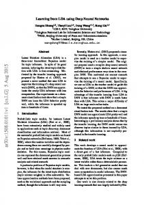
2. Convolutional neural networks Deep learning is a model that is made of multiple processing layers to learn data representation (LeCun et al., 2015). Deep learning is different from traditional neural networks, which have been used in soil spectra processing, as it involves more layers and deeper architectures. Deep neural networks allow the use of raw or unprocessed data (e.g. images or spectra) and automatically discover the representations needed for prediction. The data are transformed at each layer, amplifying aspects of the input data that are important and suppressing irrelevant information for enhanced prediction. One such deep learning model is the convolutional neural network (CNN), which is a neural network that includes one or more convolutional layers in its architecture. CNN is designed to take data in the form of multiple arrays such as images. A convolutional layer performs convolutions over an array (Fig. 1) using multiple filters. These layers are connected by weights, which are learned during training. After training, each filter can identify different features, similar to an image edge detection filter (e.g.: Sobel-Feldman; Eq. 1). A single convolutional layer is capable of identifying simple features and, as more layers are added, the network is capable of extracting features of increasing complexity and abstraction (LeCun et al., 1990). Initial image

Filter

*

Resulting image

w0

w1

w3

w4

w5

w6

w7

w8

w9

=

Fig. 1: Example of the first 3 steps of a convolution of a 3x3 filter over a 5x5 array (image). The resulting pixel values correspond to the sum of the element-wise multiplication of the initial pixels (dashed lines) and the filter.

3

Shorizontal

 −1   = 0  1

−2 0 2

 −1   0 ;  1

Svertical

 −1   = −2  −1

0 0 0

 1   2  1

(1)

CNNs have been widely used in computer vision, but also in speech recognition and time-series analysis (LeCun et al., 1995). They have the capacity of exploiting local correlations (spatial, temporal or both, depending on the input data) which makes them more suitable for this type of analysis than traditional fully-connected neural networks. For more insights about CNN we refer the reader to the seminal works of LeCun et al. (1990) and Krizhevsky et al. (2012).

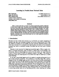
3. Spectrograms Spectrograms appeared in signal processing to visualise a sound as early as 1947, with one of the first examples shown by Potter et al. (1947). Spectrograms are a representation of a signal in a 2D space (e.g.: time-frequency for audio), where the magnitude of the signal is represented by the value of the pixels. Spectrograms are usually generated by decomposing the signal into overlapping segments to which a short-time fast Fourier transformation is applied (Griffin and Lim, 1984). To generate the spectrograms, we used a Hann window (Blackman and Tukey, 1958), a segment length of 100, with 50 observations of overlap, and a sampling frequency of one. After generating the spectrograms, they were transformed to a logarithmic scale. By processing the spectral data in this way, we generated a different (2D) representation of the spectrum which is more appropriate for our CNN (based on 2D convolutions) to process, from a vector of length 4,200 to a matrix of 51x83 (frequency x wavelength). Examples of the original data and the resulting spectrograms are shown in Fig. 2. In this new representation, it is still possible to distinguish the drops in reflectance as larger (brighter) values in a short window and wide range of frequencies, and also a subtle overall increase of values (a ”glow”) at lower levels of reflectance (Fig. 2, right panels). In effect, spectrograms automatically performed and represented multiple scaling of the spectra as in wavelet transform.

4. CNN Model Designing a CNN is a highly iterative process which includes making decisions on hyperparameter such as the number and type of layers used, and learning rate. Here we introduce a CNN model for processing spectral data and present the networks with the best performing combination of hyperparameters. 4.1. Network architecture The CNN follow a series of combinations of convolution and pooling layers (Table 1). Units in a convolutional layer are organised in feature maps (here we used 3x3). A feature map, represented as a 4

Frequency Reflectance

0.5

0.5

0.4

0.4

0.3

0.3

0.2

0.2

0.1

0.1

0.0

0.0

0.7

0.7

0.6

0.6

0.5

0.5

0.4

0.4

0.3

0.3

500 1000 1500 2000 2500 3000 3500 4000 Wavelength

500 1000 1500 2000 2500 3000 3500 4000 Wavelength

Fig. 2: Example of spectral data encoded as a spectrogram. Top panels: spectrogram with amplitude (colour) in log scale. Bottom panels: original spectral data. Left panels: mineral soil (0.5% organic carbon). Right panels: organic soil (20% organic carbon)

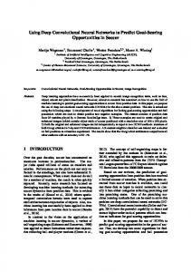
square in Fig. 1, corresponds to the output for one of the learned features which are detected at each of the image positions. Each unit of the feature map is connected to local patches in the feature maps of the previous layer through a set of weights. These locally weighted sums are then passed through a non-linear function, such as the ReLU (Rectified Learned Unit) function: f (x) = max(0, x), where x is the input to a neuron. Following the convolution layer, Max-Pooling layers combine inputs from the convolutional layers using a 2x2 window, thus reducing the resolution of the feature maps (Scherer et al., 2010). After several stages of convolution and pooling, the results are flattened (to a 1D array) and followed by fully-connected layers. These convolutional and pooling layers are based on the principles of a network mixing simple and complex cells in neuroscience. CNN takes into account the compositional hierarchies of data, e.g., local signals of spectra form peaks and valleys, and the whole forms a spectrum. Thus the idea is to extract a representation from local information at various scales to predict soil properties. As the information moves through the network, the representation changes (Fig. 3), going from an 83x51 image to the single value prediction. Table 1 summarises the architecture of the CNN used in this study. It contains seven trainable layers — five convolutional and two fully-connected layers.

5

Table 1: Sequence of layers used to build the neural network.

Type

51

Filters

Activation

Convolutional

3x3

64

ReLU

Max-Pooling

2x2

-

-

Convolutional

3x3

128

ReLU

Convolutional

3x3

256

ReLU

Max-Pooling

2x2

-

-

Convolutional

3x3

512

ReLU

Convolutional

3x3

512

ReLU

Fully-connected

-

100

ReLU

Fully-connected

-

1

Linear

100

25

51

3

Kernel size

25

3 83

41 83

128

41

12

12 20 256

512

20

1 64

64

Fig. 3: Sequence of layers showing the information flow from an input spectrogram (left end) to a single value prediction (right end).

4.2. Multi-task network CNNs have the capacity to predict multiple soil properties in a single network and training process. To utilise this capability, we used the same six soil properties and we varied the network architecture (Table 2). The new architecture has a series of four shared convolutional layers, followed by, for each property, a series of one convolutional and one fully-connected layer (Fig. 4). The head of the network (“Common layers”) is a series of convolutional and max-pooling layers. This section of the network is shared by all the target soil properties and should be able to learn how the spectrogram is structured. After the “Common layers” extract a general representation of the data represented by the spectrogram, the information is directed to 6 different branches, one for each target soil property. Each branch consists of a convolutional layer (BN) which is flattened (to 1D) before generating the output . The branches should be able to learn the signals found in the spectrogram that are specific for each soil property. The effect of using a multi-task model has been widely studied. In a review by Ruder (2017), it is mentioned that using a multi-task model reduces the risk of overfitting (by using additional information, 6

Table 2: Sequence of layers used to build the multi-task neural network

Layer type

Kernel size

Filters

Activation

†Convolutional

3x3

64

ReLU

†Max-Pooling

2x2

-

-

†Convolutional

3x3

128

ReLU

†Convolutional

3x3

256

ReLU

†Max-Pooling

2x2

-

-

†Convolutional

3x3

512

ReLU

‡Bottle-neck

1x1

64

ReLU

-

1

Linear

‡Fully-connected

†Common layers; ‡for each property

Common layers spectrograms

conv_1

max_pool_1

conv_2

conv_3

max_pool_2

BN_OC

flatten_OC

OC

BN_CEC

flatten_CEC

CEC

BN_clay

flatten_clay

clay

BN_sand

flatten_sand

sand

BN_pH

flatten_pH

pH

BN_N

flatten_N

N

conv_4

Fig. 4: Architecture of the multi-task network. “Common layers” represent the layers shared by all the predicted properties. Each branch, one per predicted soil property, correspond to a series of one convolutional layer (BN: bottle-neck layer, which reduces the dimensionality of the data) and a fully-connected layer of size=1, which corresponds to the final prediction

acting as a regularisation) and, more notably, the accuracy increases continuously with the number of tasks (Ramsundar et al., 2015). 4.3. Training the network To find the optimal weights of the network, the network needs to be trained using the data. Usually, when using CNNs the data is processed in batches, which allows the use of big datasets that cannot fit in memory at once. One cycle through the entire training dataset is a training epoch. During the training, the weights are adjusted based on a gradient-based optimisation method, meaning that the partial derivatives of the parameters with respect to the error were evaluated and the parameters were adjusted towards a minimum error value. The rate of change of parameters along the error gradient is controlled by the learning rate. If 7

the learning rate is too high, the weights will change far too much with each iteration, which will make the parameters “bounce” around the optimal solution, or simply diverge. If the learning rate is too low, the parameters might never converge. In this work, we trained the network during 20 epochs, using a batch size of 10 and the Adam optimiser (Kingma and Ba, 2014). Adam maintains a learning rate for each parameter and modifies them during the training based on exponential decays, β1 and β2 , of the first- and second-moment of the estimates respectively. 4.4. The data We used 2 datasets to test the performance of CNN. The first is a large regional dataset (LUCAS, Stevens et al., 2013) from Europe with 19,036 topsoil (composite of five sub-samples of the top 30 cm) observations with physicochemical and biological properties from Europe (Stevens et al., 2013). Samples are distributed over all land use/cover types, with some over-representation of croplands and under-representation of Eastern Europe. The soil samples were ground and passed through a 2 mm sieve. The samples were scanned with a diffuse reflectance spectrometer (XDSTM Rapid Content Analyzer) with reflectance data from 400 to 2500 nm at a spectral resolution of 0.5 nm, resulting in 4200 wavelengths. From the LUCAS dataset, we selected six soil properties which were known to be well predicted by the VNIR spectra: a) organic carbon content (OC, g kg−1 ), b) cation exchange capacity (cmol+ kg−1 ), c) clay particle size fraction (%), d) sand particle size fraction (%), e) pH measured in water, and f ) total nitrogen content (N, g kg−1 ). A summary of statistics of these soil properties is presented in Table 3. Table 3: Summary statistics of soil properties (n=19,036) for the LUCAS Soil database (Stevens et al., 2013).

OC

CEC

Clay

Sand

pH

N

(g kg−1 )

(cmol+ kg−1 )

(%)

(%)

Minimum

0.00

0.00

0.00

1.00

3.21

0.00

Maximum

586.80

234.00

79.00

99.00

10.08

38.60

Mean

50.00

15.76

18.88

42.88

6.20

2.92

Median

20.80

12.40

17.00

42.00

6.21

1.70

St. Dev.

91.31

14.48

13.00

26.11

1.35

3.76

Skewness

3.67

4.24

0.91

0.19

-0.08

3.76

(g kg−1 )

To test the effect of dataset size, we used a second, smaller, dataset from the study of Geeves et al. (1995). The dataset represents 72 soil profiles (390 samples) in the wheat-belt of southern NSW and northern Victoria, Australia. The samples covered a range of soil types and were taken from different soil horizons up to 1 m depth. The soil samples were ground and passed through a 2 mm sieve. Samples 8

were scanned using an AgriSpecTM instrument for reflectance spectra (350–2500 nm, 1nm resolution). We selected five soil properties, namely total carbon (g kg−1 ), CEC, clay and sand content, and pH (in CaCl2 ). A summary of statistics of soil properties for these soil samples is presented in Table 4. Table 4: Summary statistics of soil properties for the dataset by Geeves et al. (1995) (n=390).

Total Carbon

CEC

Clay

Sand

pH

(g kg−1 )

(cmol+ kg−1 )

(%)

(%)

Minimum

0.06

0.40

5.00

14.00

3.76

Maximum

12.74

36.43

74.00

91.00

8.23

Mean

1.17

9.17

26.60

56.92

5.49

Median

0.85

7.34

20.00

60.00

5.32

St. Dev.

1.37

5.79

16.62

16.50

0.98

Skewness

4.22

1.40

1.02

-0.53

0.67

For the LUCAS database, we modelled organic and mineral samples together as we tried to model only using spectral data without having any prior information about the samples. The soil properties and spectra of both datasets were used here for testing the CNN model. 4.5. Training & Validation In this study, we divided the LUCAS dataset into a training set, a validation set, and a test set. The training set is used to fit or train the models; the validation set is used to estimate prediction error for parameter selection; and the test set is used to assess the error of the model. From the full dataset, 25% (n = 4,759) of the samples were randomly selected and used as a test set. The rest of the data were used in training and validation. We performed a bootstrapping routine (Efron and Tibshirani, 1993) with 100 repetitions and measured the accuracy of a prediction by generating different models from different realisations of the data. A bootstrapping routine assumes that the training data set is a representation of the population, and multiple realisations of the population can be simulated from a single dataset. This is done by repeated random “sampling with replacement” of the original dataset of size 14,277 to obtain 100 bootstraps, each of size 14,277. Theoretically, about 2/3 of the data will be used in training in a bootstrap iteration, and the remaining 1/3 of data is used as validation. And thus we have a 50:25:25 percent split of data into training, validation, and test sets. For all datasets, and at each bootstrap iteration, we estimated the root mean squared error (RMSE), coefficient of determination (R2 ), mean error (ME) of prediction, and concordance correlation coefficient (ρc ; Lawrence and Lin, 1989). 9

To compare our results with conventional techniques, we generated predictive models using a Cubist regression tree (Quinlan et al., 1992) and Partial Least Squares regression (PLS; Martens and Naes, 1989) model, which are commonly used in soil spectroscopy studies (Brown et al., 2006; Minasny and McBratney, 2008; Stevens et al., 2013; Niazi et al., 2015; Viscarra Rossel et al., 2016). Before training the Cubist and PLS models, the spectral data were pre-processed using a series of methods commonly used in the literature: a) converting reflectance to apparent absorbance (a = −log10 (r)); b) Savitzky–Golay smoothing (Savitzky and Golay, 1964), using a window size of 11, and a second order polynomial; c) edges trimming (< 500 nm and > 2450 nm) to discard noisy data; d) sampling every tenth measurement; and e) applying a standard normal variate transformation (Barnes et al., 1989). For the small dataset (Geeves et al., 1995), the data were randomly split into training/validation sets during the bootstrapping routine. Considering the small number of samples, we did not perform a training/validation/testing split. We used a similar network like the one described in Table 1 but with some minor modifications to avoid overfitting. We replaced the first fully-connected layer with a dropout rate (Nitish et al., 2014) with a probability of 0.5. As a reference, we also compared the results with the Cubist model. 4.6. Implementation The CNN was implemented in Python (v3.6.2; Python Software Foundation, 2017) using Keras (v2.1.2; Chollet et al., 2015) and Tensorflow (v1.4.1; Abadi et al., 2015) backend. The Cubist and PLS models were implemented in R (v3.3.1; R Core Team, 2016), using the packages Cubist (v0.2.1; Kuhn and Quinlan, 2017) and pls (v2.6-0; Mevik et al., 2016) respectively. Computing was done using the University of Sydney’s Artemis high performance computing facility.

5. Results and discussion 5.1. Training To evaluate the effectiveness of the CNN model in predicting soil properties, we listed the performance of the model (Table 5) which shows good results, with mean R2 ranging from 0.63 for sand to 0.94 for OC. Not surprisingly, the performance in the training datasets is better than on the test and validation datasets. The models do not overfit, as shown by the similar performance between the training and validation datasets. The similarity in the error of training, validation, and test sets is also a sign of good hyperparameter selection. The estimates are slightly biased, however, the bias is generally less than 10% of the minimum values of the properties (Table 3). The observed errors are comparable with the results reported by Stevens et al. (2013) who used a variety of machine learning prediction algorithms for the prediction of OC on the same dataset. The study by 10

Table 5: Training statistics using multi-task CNN for OC (g kg−1 ), CEC (cmol+ kg−1 ), clay content (%), sand content (%), pH and N (g kg−1 ). Mean, standard deviation (sd), minimum (min) and maximum (max) of 100 bootstrap realisations.

Train (n = 50%)

Validation (n = 25%)

Test (n = 25%)

RMSE

R2

ME

RMSE

R2

ME

RMSE

R2

ME

mean

24.75

0.94

-0.79

29.78

0.90

-0.45

28.83

0.90

-1.29

sd

2.66

0.01

1.12

1.82

0.01

1.10

1.63

0.01

1.40

min

20.26

0.93

-1.58

27.73

0.89

-1.23

26.93

0.89

-2.28

max

28.25

0.96

0.00

33.38

0.91

0.32

31.86

0.91

-0.31

mean

7.75

0.74

2.34

8.52

0.66

2.21

8.68

0.65

2.10

sd

0.40

0.03

0.26

0.21

0.02

0.15

0.47

0.02

0.33

min

7.29

0.68

2.16

8.18

0.63

2.11

7.97

0.62

1.86

max

8.32

0.77

2.53

8.84

0.70

2.32

9.65

0.68

2.33

mean

6.46

0.77

-0.53

7.37

0.69

-0.61

7.47

0.68

-0.65

sd

0.53

0.03

2.75

0.34

0.02

2.94

0.26

0.02

2.86

min

5.65

0.72

-2.47

6.78

0.67

-2.69

7.06

0.65

-2.67

max

7.07

0.81

1.41

7.85

0.73

1.47

7.78

0.70

1.37

mean

15.86

0.63

-1.53

17.85

0.54

-1.30

18.03

0.54

-1.16

sd

1.75

0.08

0.61

0.65

0.03

0.51

0.59

0.02

0.60

min

12.09

0.53

-1.96

17.01

0.50

-1.67

17.21

0.50

-1.58

max

17.97

0.80

-1.10

18.75

0.57

-0.94

19.01

0.57

-0.73

mean

0.44

0.90

0.04

0.49

0.87

0.04

0.50

0.87

0.04

sd

0.02

0.01

0.02

0.01

0.00

0.02

0.01

0.00

0.02

min

0.42

0.89

0.02

0.48

0.87

0.03

0.49

0.86

0.02

max

0.46

0.91

0.05

0.52

0.88

0.05

0.52

0.87

0.06

mean

1.30

0.89

-0.19

1.51

0.85

-0.21

1.52

0.83

-0.22

sd

0.05

0.01

0.18

0.06

0.01

0.14

0.04

0.01

0.17

min

1.22

0.88

-0.32

1.45

0.84

-0.31

1.47

0.81

-0.34

max

1.38

0.90

-0.07

1.63

0.86

-0.11

1.59

0.85

-0.10

OC

CEC

Clay

Sand

pH

N

Stevens et al. (2013) partitioned the data by landuse or organic/mineral soil types, and they obtained best calibrations with a R2 of 0.76 and 0.78 for mineral and organic soils, respectively. 5.2. Multi-tasking prediction Fig. 5 shows the evolution of the error when predicting more properties in a single model. For most properties, we can observe a decrease in the error, ranging from 20.6% for sand content to 74.4% for total 11

N, when we predicted all six properties simultaneously. This behaviour is similar to what Ramsundar et al. (2015) described in their drug discovery study, where accuracy increased continuously with the number of tasks. In the case of pH, there was an increase of the error by 8.3%. Accepting this trade-off will depend on the application. In this case, we think that an increase in the RMSE of 0.04 pH units is acceptable considering the improvements in the predictions of the other properties. OC

10.0% 0.0%

29.16

0.0%

15.31

CEC

Clay 0.0%

-10.0%

-10.0%

-20.0%

-10.0%

-20.0%

-30.0%

-20.0%

-30.0%

-40.0%

-30.0%

-40.0%

-50.0%

-40.0%

-50.0%

-60.0% Sand

0.0% -10.0% -20.0% -30.0%

26.00

pH 10.0% 8.0% 6.0% 4.0% 2.0% 0.0% -2.0% -4.0% -6.0%

0.0%

7.45

3.75

N

-10.0% -20.0% -30.0% -40.0% -50.0%

0.50

-60.0% -70.0%

Fig. 5: Percentage change in error when more properties are predicted simultaneously. X-axes correspond to the number of extra variables used, starting from zero. Value next to the first point corresponds to the RMSE when only the target property is used. Error bars correspond to the 90% confidence interval after 100 iterations.

This approach provides an interesting way for simultaneous prediction of soil properties within a single model, not just in the sense of using a single spectrum for the characterisation of various soil properties (Islam et al., 2003), but as a truly synergistic model. When the network is predicting a property, it uses the rest of the predicted properties as “hints” that constrain or enhance the prediction. A simplified example is in the case of clay and sand content. If the model is predicting a very high clay content, there is an indication that the sand content should be low. The interactions between 6 properties are more complex, but the decrease in the prediction error when including more soil properties in the prediction, as shown in Fig. 5, is an indicator that the network is generating these interaction rules. 5.3. CNN vs conventional prediction techniques To gauge the performance of our CNN, we compared its performance with techniques commonly used in soil spectroscopy literature (Table 6), i.e. PLS regression and Cubist regression tree. A graphical summary 12

of the performance of all models is shown in Fig. 6. In general, PLS was the worst performing model. Cubist generally presented an excellent performance in the training dataset, but the training/validation error ratio was higher compared with CNN (Cubist: 1.7; CNN single: 1.1; CNN multi: 1.4) which translates into a poorer performance when dealing with data different from the training dataset. The CNN model, when predicting a single property, tended to generalise better in the training dataset, showing a more similar performance between the training and validation dataset. In the multi-task approach, the CNN performed better than the single prediction (as shown in Fig. 5) and usually better than the Cubist model. Table 6: Comparison of the performance of all methods for the test dataset for OC (g kg−1 ), CEC (cmol+ kg−1 ), clay content (%), sand content (%), pH and N (g kg−1 ).

RMSE

PLS

Cubist

CNN

CNN multi

130.50

43.75

32.14

16.82

2

R

0.35

0.79

0.88

0.69

ME

-3.97

-2.23

-2.28

2.25

ρc

0.52

0.89

0.94

0.83

RMSE

OC

13.60

11.34

8.58

6.51

2

R

0.23

0.41

0.66

0.63

ME

-1.47

0.06

1.86

-0.87

ρc

0.47

0.64

0.75

0.77

RMSE

CEC

8.75

10.67

7.55

7.29

2

R

0.55

0.42

0.70

0.68

ME

-0.53

-0.16

-2.67

-0.18

ρc

0.71

0.64

0.81

0.81

RMSE

Clay

19.49

22.09

18.15

17.00

2

R

0.44

0.38

0.53

0.59

ME

-0.45

1.00

-1.58

-0.45

ρc

0.63

0.62

0.70

0.76

RMSE

Sand

0.61

0.68

0.50

0.53

2

R

0.80

0.77

0.87

0.84

ME

0.02

0.02

0.06

-0.08

ρc

0.89

0.87

0.93

0.91

RMSE

pH

3.21

2.37

1.54

1.06

2

R

0.43

0.64

0.83

0.60

ME

-0.42

-0.08

-0.34

0.01

ρc

0.65

0.80

0.90

0.77

N

13

OC

175

Clay

18

150

9

16

125 RMSE

CEC

20

8

14

100

12

7

75

10

6

50

8

25

6

0

5 4

4 PLS

Cubist

CNN_single

CNN_multi

Sand

PLS

Cubist

CNN_multi

18 16 14

6

0.50

5

0.45

4

PLS

Cubist

CNN_single

CNN_multi

0.30

CNN_multi Training Validation Test

7

0.55

3 2

0.35

10

CNN_single

8

0.40

12

Cubist

N

0.60

20

PLS

pH

0.65

22

CNN_single

1 PLS

Cubist

CNN_single

CNN_multi

PLS

Cubist

CNN_single

CNN_multi

Fig. 6: Comparison between PLS, Cubist and CNN for OC (g kg−1 ), CEC (cmol+ kg−1 ), clay content (%), sand content (%), pH and N (g kg−1 ).

Based on the test dataset (Table 6), Cubist performed better than PLS except for sand and pH. Notably, Cubist showed a relative improvement (calculated as the RMSE difference over PLS) of 67% for OC. All individual CNN models performed better than PLS and Cubist. Compared with Cubist, the single-prediction CNN model reduced RMSE by 26.5, 24.4, 29.3, 17.9, 26.4, and 34.9% for OC, CEC, clay, sand, pH and total N, respectively. The multi-task CNN further improved over Cubist by 61.6, 42.6, 31.7, 23.0, 22.3, and 55.4% for the same soil properties. The total improvement of the multi-task CNN over PLS was 87.1, 52.1, 16.7, 12.8, 13.1, and 67.0%. Such dramatic improvements are rarely found in the soil spectroscopy literature. For example, in Stevens et al. (2013) study for OC prediction, the maximum difference in RMSE for different machine learning methods is about 20%. OC is usually the focus of many soil spectroscopy studies (Dalal and Henry, 1986; Ben-Dor and Banin, 1995; Chang et al., 2001; McCarty et al., 2002; Wills et al., 2014) given that it is a key component of functional ecosystems and crucial for food, soil, water and energy security (Stockmann et al., 2015; Minasny et al., 2017). The multi-task CNN is able to substantially improve the prediction compared with traditional methods, over a wide range of soils, which makes it an interesting candidate for rapid soil carbon assessment model in a regional or global context. It is also worth mentioning that the CNN models were trained with little spectral pre-treatment, we used the full reflectance spectra, and utilised all the multiscale variation represented by the spectrogram. We 14

believe that the CNN is able to select the best spectra representation based on various smoothing scales. Previous approaches require decomposition of the spectra using wavelets, and selecting wavelet coefficients to produce parsimonious multivariate calibrations (Viscarra Rossel and Lark, 2009). CNN is known to outperform conventional prediction techniques and this has been found in different disciplines (LeCun et al., 2015). Our findings also agree with the study of Bjerrum et al. (2017), which compared PLS and CNN models on spectral data in chemometrics. 5.4. Dataset size Machine learning, and especially deep learning, is a very data-hungry approach. Our proposed method has proved to work well with a heterogeneous training dataset of around 10,000 samples (considering that 25% of the initial dataset was excluded as a test set, and approximately 1/3 of data not sampled by the bootstrapping routine and used as an internal validation set). However, local soil spectroscopy datasets are generally much smaller, and thus we tested our proposed method on a smaller dataset of 390 soil samples. For all the methods, the R2 values (Table 7) were within an expected range. The RMSE values (Fig. 7) showed a good performance of CNN predicting a single property. In comparison with the Cubist model, the trend is similar to the one observed in the LUCAS dataset (Fig. 6), with Cubist performing better in the training set and with a greater training/validation error ratio (Cubist: 2.7; CNN single: 1.6; CNN multi: 1.0). Total Carbon 20

Clay

35 30

10

15 RMSE

CEC

12

25

8

20 6

10

15

4 5

10

2 Cubist

CNN_single

CNN_multi

5 Cubist

CNN_single

CNN_multi

0

Cubist

CNN_single

pH (CaCl2)

Sand 60

5

50

Training Validation

4

40 3

30

2

20

1

10 0

Cubist

CNN_single

CNN_multi

0

Cubist

CNN_single

CNN_multi

Fig. 7: Comparison of error (100 iterations) between training and validation sets for the small dataset.

15

CNN_multi

Table 7: Comparison of the coefficient of determination (mean R2 for 100 iterations) of all methods for the small dataset (validation set).

Cubist

CNN single

CNN multi

Total Carbon

0.79

0.79

0.77

CEC

0.74

0.78

0.77

Clay

0.70

0.73

0.72

Sand

0.62

0.58

0.58

pH (CaCl2 )

0.57

0.59

0.58

We want to draw the attention to the performance of the multi-task CNN. For all properties, the performance is worse than the Cubist model, probably due to the lack of information (small number of samples) when trying to generalise. This agrees with the general consensus in deep learning that dataset size matters. Despite this fact, it is possible that this behaviour will vary for small, more homogeneous datasets.

6. Conclusions We successfully applied a CNN model to predict six soil properties from raw spectral data. The only data pre-treatment used was representing the raw spectral data as a spectrogram, a technique not commonly used in soil spectroscopy and, compared with the traditional pre-treatments, very simple to apply. We also explored the capacity of CNN to be trained in a multi-task setting. This allowed the simultaneous (with one model) prediction of six soil properties from a single spectrum. This has obvious implications in simplicity and computing time, but also the capacity to achieve synergy, usually improving the predictions compared with a single property prediction. This has an interesting potential, especially for large soil spectroscopy projects where the spectral data usually goes along with laboratory measurements of multiple soil properties. The proposed approach performs better than the traditional PLS regression and Cubist models, which are the most commonly used models for soil spectroscopy. In our study, the multi-task approach significantly reduced the error compared to the Cubist model, notably by 61.6 and 55.4% for organic carbon and total nitrogen, respectively. Such dramatic improvement is rarely found in spectroscopy studies. We observed that the multi-task CNN was not effective on a smaller dataset. Our approach showed worse performance than the traditional Cubist model. This is not surprising as deep learning is a very data-hungry approach. This fact has been widely recognised by the deep learning community, which, up to this point, agrees that dataset size matters. 16

Deep learning is an exciting discipline that has already changed many fields, including computer vision, natural language processing, medical image analysis, etc. This paper shows how deep learning has the potential to change the way we model soil spectral data. 7. Acknowledgements We acknowledge the work of all the scientists who generated and made available the two spectral datasets used in this study. This research was supported by Sydney Informatics Hub, funded by the University of Sydney. References Abadi, M., Agarwal, A., Barham, P., Brevdo, E., Chen, Z., Citro, C., Corrado, G. S., Davis, A., Dean, J., Devin, M., Ghemawat, S., Goodfellow, I., Harp, A., Irving, G., Isard, M., Jia, Y., Jozefowicz, R., Kaiser, L., Kudlur, M., Levenberg, J., Man´ e, D., Monga, R., Moore, S., Murray, D., Olah, C., Schuster, M., Shlens, J., Steiner, B., Sutskever, I., Talwar, K., Tucker, P., Vanhoucke, V., Vasudevan, V., Vi´ egas, F., Vinyals, O., Warden, P., Wattenberg, M., Wicke, M., Yu, Y. & Zheng, X. (2015). TensorFlow: Large-Scale Machine Learning on Heterogeneous Systems. Software available from tensorflow.org. URL https://www.tensorflow.org/ Barnes, R., Dhanoa, M. S. & Lister, S. J. (1989). Standard normal variate transformation and de-trending of near-infrared diffuse reflectance spectra. Applied spectroscopy 43 (5), 772–777. Bellon-Maurel, V. & McBratney, A. (2011). Near-infrared (NIR) and mid-infrared (MIR) spectroscopic techniques for assessing the amount of carbon stock in soils–Critical review and research perspectives. Soil Biology and Biochemistry 43 (7), 1398–1410. Ben-Dor, E. & Banin, A. (1995). Near-infrared analysis as a rapid method to simultaneously evaluate several soil properties. Soil Science Society of America Journal 59 (2), 364–372. Bengio, Y. (2012). Deep learning of representations for unsupervised and transfer learning. In: Proceedings of ICML Workshop on Unsupervised and Transfer Learning. pp. 17–36. Bjerrum, E. J., Glahder, M. & Skov, T. (2017). Data Augmentation of Spectral Data for Convolutional Neural Network (CNN) Based Deep Chemometrics. arXiv preprint arXiv:1710.01927. Blackman, R. B. & Tukey, J. W. (1958). The measurement of power spectra. Brown, D. J., Shepherd, K. D., Walsh, M. G., Mays, M. D. & Reinsch, T. G. (2006). Global soil characterization with VNIR diffuse reflectance spectroscopy. Geoderma 132 (3), 273–290. Chang, C.-W., Laird, D. A., Mausbach, M. J. & Hurburgh, C. R. (2001). Near-infrared reflectance spectroscopy–principal components regression analyses of soil properties. Soil Science Society of America Journal 65 (2), 480–490. Chen, Y., Lin, Z., Zhao, X., Wang, G. & Gu, Y. (2014). Deep learning-based classification of hyperspectral data. IEEE Journal of Selected topics in applied earth observations and remote sensing 7 (6), 2094–2107. Chollet, F. et al. (2015). Keras. https://github.com/fchollet/keras. Dalal, R. & Henry, R. (1986). Simultaneous Determination of Moisture, Organic Carbon, and Total Nitrogen by Near Infrared Reflectance Spectrophotometry 1. Soil Science Society of America Journal 50 (1), 120–123. Efron, B. & Tibshirani, R. J. (1993). An introduction to the bootstrap. Vol. 57. CRC press, New York. Geeves, G., Cresswell, H., Murphy, B., Gessler, P., Chartres, C., Little, I. & Bowman, G. (1995). The physical, chemical and morphological properties of soils in the wheat-belt of southern New South wales and northern Victoria. NSW Department of Conservation and Land Management.

17

Gras, J.-P., Barth` es, B. G., Mahaut, B. & Trupin, S. (2014). Best practices for obtaining and processing field visible and near infrared (VNIR) spectra of topsoils. Geoderma 214, 126–134. Griffin, D. & Lim, J. (1984). Signal estimation from modified short-time Fourier transform. IEEE Transactions on Acoustics, Speech, and Signal Processing 32 (2), 236–243. Islam, K., Singh, B. & McBratney, A. (2003). Simultaneous estimation of several soil properties by ultra-violet, visible, and near-infrared reflectance spectroscopy. Soil Research 41 (6), 1101–1114. Kingma, D. & Ba, J. (2014). Adam: A method for stochastic optimization. arXiv preprint arXiv:1412.6980. Krizhevsky, A., Sutskever, I. & Hinton, G. E. (2012). Imagenet classification with deep convolutional neural networks. In: Advances in neural information processing systems. pp. 1097–1105. Kuhn, M. & Quinlan, R. (2017). Cubist: Rule- And Instance-Based Regression Modeling. R package version 0.2.1. URL https://CRAN.R-project.org/package=Cubist Lawrence, I. & Lin, K. (1989). A concordance correlation coefficient to evaluate reproducibility. Biometrics, 255–268. LeCun, Y., Bengio, Y. & Hinton, G. (2015). Deep learning. Nature 521 (7553), 436–444. LeCun, Y., Bengio, Y. et al. (1995). Convolutional networks for images, speech, and time series. The handbook of brain theory and neural networks 3361 (10), 1995. LeCun, Y., Boser, B. E., Denker, J. S., Henderson, D., Howard, R. E., Hubbard, W. E. & Jackel, L. D. (1990). Handwritten digit recognition with a back-propagation network. In: Advances in neural information processing systems. pp. 396–404. Martens, H. & Naes, T. (1989). Multivariate calibration. John Wiley & Sons. McCarty, G., Reeves, J., Reeves, V., Follett, R. & Kimble, J. (2002). Mid-infrared and near-infrared diffuse reflectance spectroscopy for soil carbon measurement. Soil Science Society of America Journal 66 (2), 640–646. Mevik, B.-H., Wehrens, R. & Liland, K. H. (2016). pls: Partial Least Squares and Principal Component Regression. R package version 2.6-0. URL https://CRAN.R-project.org/package=pls Minasny, B., Malone, B. P., McBratney, A. B., Angers, D. A., Arrouays, D., Chambers, A., Chaplot, V., Chen, Z.-S., Cheng, K., Das, B. S. et al. (2017). Soil carbon 4 per mille. Geoderma 292, 59–86. Minasny, B. & McBratney, A. B. (2008). Regression rules as a tool for predicting soil properties from infrared reflectance spectroscopy. Chemometrics and intelligent laboratory systems 94 (1), 72–79. Morellos, A., Pantazi, X.-E., Moshou, D., Alexandridis, T., Whetton, R., Tziotzios, G., Wiebensohn, J., Bill, R. & Mouazen, A. M. (2016). Machine learning based prediction of soil total nitrogen, organic carbon and moisture content by using VIS-NIR spectroscopy. Biosystems Engineering 152, 104–116. Niazi, N. K., Singh, B. & Minasny, B. (2015). Mid-infrared spectroscopy and partial least-squares regression to estimate soil arsenic at a highly variable arsenic-contaminated site. International Journal of Environmental Science and Technology 12 (6), 1965–1974. Nitish, S., Hinton, G. E., Krizhevsky, A., Sutskever, I. & Salakhutdinov, R. (2014). Dropout: a simple way to prevent neural networks from overfitting. Journal of machine learning research 15 (1), 1929–1958. Potter, R., Kopp, G. & Green, H. (1947). Visible Speech. Van Nostrand, New York. Python Software Foundation (2017). Python Language Reference. Python Software Foundation. URL https://www.python.org Quinlan, J. R. et al. (1992). Learning with continuous classes. In: 5th Australian joint conference on artificial intelligence. Vol. 92. Singapore, pp. 343–348. R Core Team (2016). R: A Language and Environment for Statistical Computing. R Foundation for Statistical Computing, Vienna, Austria. URL https://www.R-project.org/

18

Ramsundar, B., Kearnes, S., Riley, P., Webster, D., Konerding, D. & Pande, V. (2015). Massively multitask networks for drug discovery. arXiv preprint arXiv:1502.02072. Romero, D. J., Ben-Dor, E., Demattˆ e, J. A., e Souza, A. B., Vicente, L. E., Tavares, T. R., Martello, M., Strabeli, T. F., da Barros, P. P. S., Fiorio, P. R. et al. (2018). Internal soil standard method for the Brazilian soil spectral library: Performance and proximate analysis. Geoderma 312, 95–103. Ruder, S. (2017). An overview of multi-task learning in deep neural networks. arXiv preprint arXiv:1706.05098. Sarathjith, M., Das, B. S., Wani, S. P. & Sahrawat, K. L. (2016). Variable indicators for optimum wavelength selection in diffuse reflectance spectroscopy of soils. Geoderma 267, 1–9. Savitzky, A. & Golay, M. J. (1964). Smoothing and differentiation of data by simplified least squares procedures. Analytical chemistry 36 (8), 1627–1639. Scherer, D., M¨ uller, A. & Behnke, S. (2010). Evaluation of pooling operations in convolutional architectures for object recognition. Artificial Neural Networks–ICANN 2010, 92–101. Shepherd, K. D. & Walsh, M. G. (2002). Development of reflectance spectral libraries for characterization of soil properties. Soil science society of America journal 66 (3), 988–998. Soriano-Disla, J. M., Janik, L. J., Viscarra Rossel, R. A., Macdonald, L. M. & McLaughlin, M. J. (2014). The performance of visible, near-, and mid-infrared reflectance spectroscopy for prediction of soil physical, chemical, and biological properties. Applied Spectroscopy Reviews 49 (2), 139–186. Stenberg, B., Rossel, R. A. V., Mouazen, A. M. & Wetterlind, J. (2010). Chapter five-visible and near infrared spectroscopy in soil science. Advances in agronomy 107, 163–215. Stevens, A., Nocita, M., T´ oth, G., Montanarella, L. & van Wesemael, B. (2013). Prediction of soil organic carbon at the European scale by visible and near infrared reflectance spectroscopy. PloS one 8 (6), e66409. Stockmann, U., Padarian, J., McBratney, A., Minasny, B., de Brogniez, D., Montanarella, L., Hong, S. Y., Rawlins, B. G. & Field, D. J. (2015). Global soil organic carbon assessment. Global Food Security 6, 9–16. Vaˇs´ at, R., Kodeˇsov´ a, R., Klement, A. & Bor˘ uvka, L. (2017). Simple but efficient signal pre-processing in soil organic carbon spectroscopic estimation. Geoderma 298, 46–53. Viscarra Rossel, R. & Behrens, T. (2010). Using data mining to model and interpret soil diffuse reflectance spectra. Geoderma 158 (1), 46–54. Viscarra Rossel, R., Behrens, T., Ben-Dor, E., Brown, D., Demattˆ e, J., Shepherd, K., Shi, Z., Stenberg, B., Stevens, A., Adamchuk, V. et al. (2016). A global spectral library to characterize the world’s soil. Earth-Science Reviews 155, 198–230. Viscarra Rossel, R., Cattle, S. R., Ortega, A. & Fouad, Y. (2009). In situ measurements of soil colour, mineral composition and clay content by vis–NIR spectroscopy. Geoderma 150 (3-4), 253–266. Viscarra Rossel, R. & Lark, R. (2009). Improved analysis and modelling of soil diffuse reflectance spectra using wavelets. European Journal of Soil Science 60 (3), 453–464. Wills, S., Loecke, T., Sequeira, C., Teachman, G., Grunwald, S. & West, L. T. (2014). Overview of the US rapid carbon assessment project: sampling design, initial summary and uncertainty estimates. In: Soil carbon. Springer, pp. 95–104.

19