Atmos. Meas. Tech., 8, 183–194, 2015 www.atmos-meas-tech.net/8/183/2015/ doi:10.5194/amt-8-183-2015 © Author(s) 2015. CC Attribution 3.0 License.
Using digital image processing to characterize the Campbell–Stokes sunshine recorder and to derive high-temporal resolution direct solar irradiance A. Sanchez-Romero1 , J. A. González1 , J. Calbó1 , and A. Sanchez-Lorenzo1,2 1 Department 2 Pyrenean
of Physics, University of Girona, Girona, Spain Institute of Ecology, Spanish National Research Council (CSIC), Zaragoza, Spain
Correspondence to: A. Sanchez-Romero (
[email protected]) Received: 30 July 2014 – Published in Atmos. Meas. Tech. Discuss.: 17 September 2014 Revised: 13 November 2014 – Accepted: 2 December 2014 – Published: 12 January 2015
Abstract. The Campbell–Stokes sunshine recorder (CSSR) has been one of the most commonly used instruments for measuring sunshine duration (SD) through the burn length of a given CSSR card. Many authors have used SD to obtain information about cloudiness and solar radiation (by using Ångström–Prescott type formulas), but the burn width has not been used systematically. In principle, the burn width increases for increasing direct beam irradiance. The aim of this research is to show the relationship between burn width and direct solar irradiance (DSI) and to prove whether this relationship depends on the type of CSSR and burning card. A method of analysis based on image processing of digital scanned images of burned cards is used. With this method, the temporal evolution of the burn width with 1 min resolution can be obtained. From this, SD is easily calculated and compared with the traditional (i.e., visual) determination. The method tends to slightly overestimate SD, but the thresholds that are used in the image processing could be adjusted to obtain an improved estimation. Regarding the burn width, experimental results show that there is a high correlation between two different models of CSSRs, as well as a strong relationship between burn widths and DSI at a hightemporal resolution. Thus, for example, hourly DSI may be estimated from the burn width with higher accuracy than based on burn length (for one of the CSSR, relative root mean squared error is 24 and 30 %, respectively; mean bias error is −0.6 and −30.0 W m−2 , respectively). The method offers a practical way to exploit long-term sets of CSSR cards to create long time series of DSI. Since DSI is affected by atmospheric aerosol content, CSSR records may also become
a proxy measurement for turbidity and atmospheric aerosol loading.
1
Introduction
Sunshine duration (SD) is a useful indicator of the amount of solar radiation arriving on the earth and a key variable for various sectors, including tourism, public health, agriculture, and energy. According to the World Meteorological Organization (WMO, 2008), the SD for a given period is defined as the total time length of those sub-periods for which the direct solar irradiance exceeds 120 W m−2 . For climatological purposes, the units used are “hours per day” as well as percentage quantities such as “relative daily sunshine duration”, where SD is divided by the maximum possible SD (i.e., as if sky was clear and a bright sun was present during the entire day, from sunrise to sunset). One of the most used instruments to measure SD is the Campbell–Stokes sunshine recorder (CSSR). It was invented in the late 19th century to provide a measurement of the duration of bright sunlight by making a burn mark on a piece of specially treated cardboard. The measurement of the length of the burn for a given card gives daily SD. For details on the history of the CSSR, we refer to Stanhill (2003) and SanchezLorenzo et al. (2013). In brief, the main parts of a current CSSR are a sphere made of transparent glass and a rounded metal frame placed behind the sphere. The glass sphere is designed to focus the Sun’s rays onto a piece of recording cardboard. The metal frame part has three overlapping sets
Published by Copernicus Publications on behalf of the European Geosciences Union.
184
A. Sanchez-Romero et al.: Using digital image processing to characterize the CSSR
of grooves to hold the recording cards for the winter, summer, and spring/autumn periods. The recording card has to be replaced daily after sunset. Different designs of cards exist with hourly and half-hourly divisions marked across these cards, enabling determination of the times of sunshine, and an estimated resolution of 0.1 h. For further details on the instrument and instructions for obtaining uniform results, as well as other traditional instruments for measuring SD, see Middleton (1969) and WMO (2008). Over the last few years, various automated instruments and other methods for obtaining SD have been developed, which are summarized in WMO (2008). One of these is the pyrheliometric method, which is based on direct irradiance measurements (e.g., Hinssen, 2006; Hinssen and Knap, 2007; Vuerich et al., 2012). Another way of determining SD is by means of automatic instruments specifically designed to this end, which have become commercially available (Wood et al., 2003; Kerr and Tabony, 2004; Matuszko, 2014). These instruments detect direct solar radiation and count the time interval during which the irradiance exceeds a certain threshold. Progressively, many weather stations have changed traditional manual instruments (such as CSSR and Jordan photographic recorders) to these automatic systems. Moreover, different methods exist nowadays to estimate SD from geostationary satellite data, which potentially provide improved spatial coverage and representativeness (Olseth and Skartveit, 2001; Good, 2010; Kothe et al., 2013). Despite the fact that new models of sunshine recorders do not require daily attention by an observer and their data reduction (i.e., the process of recording and storing the SD data) is faster and more accurate, there is a consensus with regard to preserving CSSR type instruments at long-established (in some cases more than 120 years ago), well-maintained, and freely exposed meteorological stations (Stanhill, 2003; Wood and Harrison, 2011; Sanchez-Lorenzo et al., 2013). A change of the instrument used to measure SD can affect the homogeneity of the data series. This may lead to significant errors when evaluating trends and may hinder the possibility of determining long-term secular trends (Powell, 1983; Steurer and Karl, 1991; Brázdil et al., 1994; Stanhill and Cohen, 2008). Among the studies that analyze long series of SD, some works choose to restrict the period in order to avoid instrumental changes, therefore not encompassing the entire period of observation (Angell et al., 1984). Other studies assess the homogeneity of the SD series, such as research conducted in the United States (Cerveny and Balling, 1990; Stanhill and Cohen, 2005), United Kingdom (Kerr and Tabony, 2004), Iberian Peninsula (Guijarro, 2007; SanchezLorenzo et al., 2007), Japan (Katsuyama, 1987; Stanhill and Cohen, 2008), China (Xia, 2010), and Switzerland (SanchezLorenzo and Wild, 2012). The results of these studies point towards the need for further research, including homogenization of the long-term SD series and the necessity of simulta-
Atmos. Meas. Tech., 8, 183–194, 2015
neous measurements by both traditional and automatic instrumentation (Aguilar et al., 2003). Differences between types of SD measurements might be attributed to their particular characteristics and limitations. As the longer SD series are generally measured using CSSR, the errors connected with this instrument are well-described (Painter, 1981; Brázdil et al., 1994). The two major problems with CSSR when comparing their measurements with other methods or instruments lie in the variability of the level of direct irradiance which produces a burn and the overburning of the card in conditions of intermittent high irradiance (Stanhill, 2003). These difficulties can be added to the obvious element of subjectivity in measuring the burn length on the CSSR cards (Brázdil et al., 1994). The problem of overburning is very difficult to evaluate as one small burst of high direct irradiance causes a burn apparently lasting far longer than the few seconds of its actual duration; standard methods have therefore been proposed to take into account this fact when evaluating the burn lengths (WMO, 2008). Despite these rules, during events of very broken cloudiness a measurement of SD by means of CSSR can be significantly overestimated (Painter, 1981; Kerr and Tabony, 2004). Regarding the first problem, defining the direct irradiance value that produces burning (“burning threshold”) is a wellknown issue. One proof is the variability of values that the WMO has given: in 1971, WMO suggested that the threshold can vary between 70 and 280 W m−2 ; in 1976, WMO recommended a threshold value of 200 W m−2 ; finally, in 1981, a value of 120 W m−2 was recommended (WMO, 2008). Gueymard (1993) tried to give some scientific justification to this value. Nevertheless, Bider (1958), Jaenicke and Kasten (1978), and Roldán et al. (2005) showed a large variety of burning thresholds for different CSSR. Similarly, Helmes and Jaenicke (1984) described the effects of using different types of recording cards. In addition, the measurement of threshold values indicated that there were notable losses of record, which must be attributed to dew or other water deposits on the glass sphere. Painter (1981) obtained monthly averaged threshold values ranging from 16 to 142 W m−2 despite some thresholds up to 400 W m−2 that were obtained in particular conditions. From the above discussion it is clear that long time series of SD include errors of several kinds and that their removal is a complicated issue. It is also important to stress that the problem of thresholds is not exclusive to the CSSR; it has been studied for other instruments such as the Foster sunshine recorder (Baker and Haines, 1969; Benson et al., 1984; Michalsky, 1992). SD series also provide additional embedded information on other magnitudes. For example, many authors relate SD for a period of time with direct and global (the sum of the solar direct and diffuse contributions) irradiance with the use of the so-called Ångström–Prescott type formulas (e.g., Sears et al., 1981; Benson et al., 1984; Martínez-Lozano et al., 1984; Stanhill, 1998; Power, 2001; Suehrcke, 2000; Bakirci, 2009), which were first proposed by Ångström (1924) and further www.atmos-meas-tech.net/8/183/2015/
A. Sanchez-Romero et al.: Using digital image processing to characterize the CSSR modified by Prescott (1940). In addition, R. Jaenicke and L. Helmes developed a series of pioneering studies presenting a method to determine atmospheric turbidity from SD records and cloud cover data (Jaenicke and Kasten, 1978; Helmes and Jaenicke, 1984, 1985, 1986) that has recently aroused interest (for a review, see Sanchez-Romero et al., 2014). SD data are also used in other fields such as agriculture (Monteith, 1977; Stanhill and Cohen, 2001) or hydrological modeling (Döll et al., 2003). This paper describes an analysis method to derive direct solar irradiance (DSI) from the CSSR burned cards by using digital image processing. The idea we assume here was first proposed by Wright (1935): the size of the burn at any point is related to the strength of the DSI focused on the card at that time. Galindo Estrada and Fournier D’Albe (1960) applied a similar approach: they compared daily values of the mass loss of burned cards (which is related to the perforation of the card and thus to mean burn width) with pyrheliometer readings. The hypothesis of using the burn width of CSSRs to obtain DSI data has recently been revisited, and several studies have shown the potential of the burn width of CSSR cards as a proxy for DSI (e.g., Wood and Harrison, 2011; Horseman et al., 2013); however, here a more complete research is presented, comparing burn width and DSI for a relatively long period of time (2 years) and investigating results at high-temporal resolution. As long-term records of SD cards are available at some historical meteorological stations, e.g., Blue Hill Observatory in United States (Magee et al., 2014; Mike Iacono, personal communication, 2014), the reconstruction of DSI for these sites can reach more than 100 years from the present day. Section 2 provides a description of data and instruments used in this research. In Sect. 3 we describe the semiautomatic method proposed for determining the width of the burned traces. In Sect. 4 we show the application of the new treatment of the CSSR cards, first to determine the daily SD and second to estimate the DSI at hourly resolution. Finally, conclusions of this study and suggestions for further research are presented in Sect. 5.
2
Instruments and data
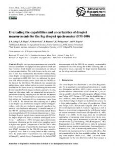
Exposed cards from CSSRs and meteorological and radiative measurements used in the present study come from a weather and radiometric station located on the roof of a building of the University of Girona (41.962◦ N, 2.829◦ E, 115 m a.s.l.). Girona is a city located in the northeast of the Iberian Peninsula, about 30 km from the Mediterranean Sea. It has a Mediterranean climate, with moderate winters and hot summers and maximum precipitation during autumn and spring. The mean height of the horizon for the CSSRs is 4.2◦ , with a minimum of 0.2◦ at azimuth angle 86◦ W and a maximum of 9.2◦ at azimuth angle 21◦ E (Fig. 1). Note that the Sun rises over the horizon at angular heights greater than 5◦ (except during summer period), while in the evening the www.atmos-meas-tech.net/8/183/2015/
185
Figure 1. Solar path for the 21st of each month (red lines) and horizon height for each azimuth angle (blue line).
Sun sets at much lower angular heights during most months. This means that the SD records and DSI measurements are slightly affected in the morning, but we assume that this issue does not affect the relationship between both variables. Two different models of CSSR have been used (Fig. 2, top panel) with three different cards for each CSSR (Fig. 2, bottom panel), which are used for different periods along the year. Hours and half-hours are printed on every card, as also shown in Fig. 2 (bottom panel). One of the CSSR and cards is from Thies Clima (hereafter referred to as CSSR1); the other CSSR is from Negretti & Zambra, manufactured in the 1980s with cards of the model Mod.98 (hereafter referred to as CSSR2), formerly used by the Spanish Meteorological Agency (AEMET). DSI is measured by a pyrheliometer (CH-1 model) from Kipp & Zonen mounted on a Sun tracker. The DSI is measured every second, and values are stored as 1 min averages. The station is also equipped with meteorological sensors to measure temperature, humidity, wind speed, precipitation, etc., as well as a ceilometer, a multifilter rotating shadowband radiometer, and other radiometric sensors. In addition, a whole sky camera is continuously taking pictures of the sky dome. We have processed 239 cards covering the period from January 2012 to January 2014 for each type of CSSR. We have 94 winter cards (from 16 October to 28/29 February), 56 equinoctial cards (from 1 March to 15 April and from 1 September to 15 October), and 89 summer cards (from 16 April to 31 August). The number of cards is limited because we did not add cards every day, and we removed the cards that were too damaged due to the rain or had no traces of burns.
3
Semiautomatic method for reading the burned traces
We have developed a semiautomatic method to retrieve information from the burned cards. We have considered “burned” not only the perforated part but also the black-grey area (scorched area) present on the edges of the burn. The method is very effective in detecting the burned areas of the CSSR cards and can be summarized in four steps. First, we scan Atmos. Meas. Tech., 8, 183–194, 2015
186
A. Sanchez-Romero et al.: Using digital image processing to characterize the CSSR dimension (2340 × 1700 pixels) for all scans. Unlike Horseman et al. (2013), we use a green background (Fig. 3a) for scanning the cards in order to obtain a contrast with the card, which is blue (face) and white (hour markers and other information). The positioning of the card on the scanner does not need to be precise, which simplifies and speeds up the card scanning process. Before the scanning, an evaluation is done to remove those cards that do not present any burn or to control for those that present any anomalies (stains on the card face, deformations due to the rain, etc.). 3.2
Figure 2. (Top) Details of the two different CSSRs mounted in Girona (NE Spain), and (bottom) an example of the 3 types of cards used during summer, winter, and equinoctial seasons, respectively (the longer the daylight hours, the longer the card): (1) summer card of Thies Clima; (2) summer card of Mod.98; (3) equinoctial card of Thies Clima (note that although the card edges are not symmetric, the markings are); (4) equinoctial card of Mod.98; (5) winter card of Thies Clima; and (6) Winter card of Mod.98.
each card on a suitable background. Second, we apply a digital process that increases the contrast of the burned area. Third, the middle of the day, 12 true solar time (TST), on the card is determined. Finally, the burn width is measured, with the help of a computer program, along cross sections spaced every minute. A schematic illustration of the different steps can also be seen in Fig. 3. With this, we obtain daily evolution of the burn width on a resolution of 1 min; the length of the burn (i.e., SD) can be easily determined. These four steps are detailed in the following sections. Our method is similar to the method of Horseman et al. (2013), but there are also significant differences that will be highlighted below. 3.1
Image treatment
On used cards, the edges of the burned or scorched traces are, for the most part, black-brown, occasionally with some grey ash. As stated by Fan and Zhang (2013), there are no abrupt changes in grey intensity between the weak scorch and the card face, but their signatures on the RGB color coordinates are noticeably different. This fact will be the basis for identifying the burned parts of the card by using the Image Processing Toolbox from MatLab on the RGB image. First, we build an image called Im1 (Fig. 3b.1), in which the pixels corresponding to the white markers in the card (hour and half-hour markers) have the value “1” and the rest of the pixels have “0”. To distinguish the white pixels, a threshold of R > 200 is applied on the red component (which ranges from 0 to 255). Then we build a second image, called Im2 (Fig. 3b.2), distinguishing the blue area of the card. The selection is made applying the condition B − R < 20 on the red and blue components. In Im2, the pixels in blue areas are labeled as “0” and all the other pixels (green, black, grey, and white) are labeled as “1”. Next, by subtracting Im1 from Im2 and setting all pixels to 0 where the difference is negative, an image with pixels labeled “1” for the burn and the background (black, grey, and green) and labeled “0” for the unburned part of the card (blue and white) is obtained. There is still some “noise” in this image (that is, pixels of one kind surrounded by eight pixels of the other kind); this noise is removed from the image to obtain the final processed image (Fig. 3c; 1 pixels in white, 0 pixels in black). Note that this process is entirely automatic. The choice of the thresholds (R > 200 for Im1 and B − R < 20 for Im2) has been empirically determined after performing various checks and will certainly affect the identification of the burn but, as long as they are used consistently throughout the two card archives, their exact absolute values are not very important.
Image capture 3.3
Similar to Horseman et al. (2013), scanning the burned card is the first step of our method and the more time-consuming manual part. For this purpose we use a commercial scanner (model HP Scanjet 5590). As sensors in image scanners alter with time and use, a method to calibrate the scanner must be applied regularly (Horseman et al., 2013). We use a standard image format, 24 bit RGB BMP (bitmap), and the same Atmos. Meas. Tech., 8, 183–194, 2015
Image positioning
Unlike Horseman et al. (2013), the positioning of the card within the image also requires some manual intervention. This is convenient for checking the scan and the image treatment and necessary to convert the image of the burned pixels into length (millimeters of width) and into time (minutes along the day). Although this step slows down the process, www.atmos-meas-tech.net/8/183/2015/
A. Sanchez-Romero et al.: Using digital image processing to characterize the CSSR 3.4
Figure 3. Steps of the semiautomatic method for retrieving information from the CSSR burned cards and for a certain day: (a) captured image, (b) treated image, (c) positioned image, and (d) measured burn width over time.
it allows using our method for any type of card. We need to manually identify two or three points (depending on the shape of the card) to find the middle of the day (12 TST). More specifically, in curved cards (summer and winter cards) we mark three points (two on the ends of the outer arc and the third close to the center of the outer arc) to find the center and the radius of the outer circumferences (the same process could be applied for the inner arc). Then, as these cards are symmetric about the midday marker, it is easy to find all points in the image belonging to the outer or inner arc and the point corresponding to noon (Fig. 3d). In the equinoctial cards, finding the midday point is even easier than in the previous ones: knowing two points (at both ends of the outer or inner contour) provides sufficient information to locate the midday point.
187
Measurement of burning width
The Horseman et al. (2013) method rectifies the image of each card (that is, images are transformed to a representation with a straight burned trace) before extracting the burn width, thus simplifying geometrical calculations. Contrarily, we consider here continuous radial sections that cover the whole card and measure the burn width (i.e., the length from the first to the last “burned” pixels) along each section. Because the size and shape of each card type is known and standardized, we know the radii of the outer and inner boundaries and their distance; thus there is no need to cross the whole image, rather just the area where the card is placed. For the equinoctial cards, parallel sections are performed instead of radial sections. We continue by defining the relation between angular (or linear) displacement and time: as we know the angle (or distance) between the two edges that we defined in the previous step, and we also know the interval of time that corresponds to these two points (this time is fixed in each type of card), the relation between angle (or distance) and time is immediate. For example, for winter and summer cards, a 1 min displacement corresponds to an angular displacement of 0.064◦ ; in the case of equinoctial cards, 1 min displacement corresponds to a linear displacement of 0.294 mm (0.317 mm) for CSSR1 (CSSR2). If we consider a resolution of one pixel, the resolution of the burn width is 0.126 mm in all cards (for the scanner used). As we know the point corresponding with 12 TST, consecutive angular displacements (corresponding to a 1 min temporal resolution) towards the left are applied, the radial sections between the inner radius to the outer radius are inspected, and the distance between the first and last “1” pixel in the radial section is computed. Thus, we obtain the temporal evolution of the burn width for the morning. We proceed in a similar way (but towards the right) to obtain the afternoon evolution of the burn width. With this, the daily evolution of the burn width in each card is finally obtained (Fig. 3e). Note that all processes in this last step are fully automatic. 4
Applications of the measurements of the burn width
The semiautomatic method proposed to process the burned cards can help in the assessment of different types of errors that can affect the SD measurements (Sect. 4.1). The method can also be useful in order to provide a record of DSI, since the burn width can be used as a proxy for pyrheliometer measurements (Sect. 4.2). 4.1
Assessment of the measurement of SD
As summarized by Brázdil et al. (1994), the sources of errors in the SD series related to the use of CSSRs are (i) the ageing of the glass ball, which with increasing operation time www.atmos-meas-tech.net/8/183/2015/
Atmos. Meas. Tech., 8, 183–194, 2015
188
A. Sanchez-Romero et al.: Using digital image processing to characterize the CSSR
Table 1. The first two columns are the mean value of SD by manual and semiautomatic methods, respectively. The third column is the value of SD from pyrheliometric method by using a DSI threshold (in parenthesis) that would approach the corresponding mean SD using the semiautomatic method. Recall that the “true” mean SD (by using 120 W m−2 as the DSI threshold) is 7.16 h.
SD1 SD2
Manual
Semiautomatic
DSI threshold
7.31 h 7.10 h
7.53 h 7.22 h
7.49 h (55 W m−2 ) 7.21 h (110 W m−2 )
becomes less transparent, (ii) the replacement of the recorder by a new device manufactured by different companies, and (iii) the variability of the recording card (e.g., different quality, color, or material). In order to homogenize the worldwide measurements of SD, a specific design of the CSSR was recommended as the reference in the 1960s (WMO, 1962). This, however, did not eliminate all the problems, especially when long-term series with records before and after the 1960s are used to study SD trends. Thus, we will here quantify these errors/differences in the observations by using our digital method applied to two different CSSRs that use different burning cards. One of the major problems when comparing SD measurements from different CSSR devices and card types is the variability of the level of DSI that produces a burn (e.g., Stanhill, 2003; Sanchez-Romero et al., 2014). Here we define the SDpyr method as considering a threshold of 120 W m−2 in DSI in order to calculate SD; that is, counting the minutes when DSI is greater than 120 W m−2 . By doing so, the mean value found for our database is 7.16 h, which can be taken as the reference (correct value) for other estimations. Table 1 shows the mean value obtained when using different methods of estimating SD applied both to CSSR1 and CSSR2. To obtain SD with the semiautomatic method described in Sect. 3 (SDaut), all minutes showing burn are counted. As shown in Fig. 4a for CSSR1, retrieved SD using the SDaut and the SDpyr methods agree very well (i.e., correlation coefficients are higher than 0.98 for both instruments), although a minor overestimation is apparent. The semiautomatic method gives a mean SD deviation with respect to SDpyr of 0.37 h (4.9 %) and 0.06 h (0.8 %) for CSSR1 and CSSR2, respectively. Although both instruments give a slight overestimation of SD, it is more pronounced for CSSR1, which shows a somewhat higher sensitivity than CSSR2. The instrument sensitivities can also be quantified by searching for the DSI threshold values that would give the corresponding mean SDaut: 55 and 110 W m−2 for CSSR1 and CSRR2, respectively; these threshold values are lower than the 120 Wm−2 suggested by the WMO. Therefore, there is some overestimation in the SD given by SDaut, which was expected because some instructions and recommendations (WMO, 2008) are not applied in the Atmos. Meas. Tech., 8, 183–194, 2015
Figure 4. Scatter plots of the (a) daily SD obtained for CSSR1 from both SDaut (blue crosses) and SDman (red points) methods against SDpyr, considering the threshold of 120 W m−2 in DSI; and (b) the daily SD obtained by the two CSSR using the automatic method. In each graphic we also represent the 1 : 1 line (black line).
method. For example, when SD is retrieved by reading the cards manually (SDman), the time length is reduced at each end by an amount equal to half the radius of curvature of the end of the burn in the case of a clear burn with round ends; on the other hand, an amount of 0.1h is subtracted from the total length of the burned segment in the case of a clear burn that is temporarily reduced in width by at least one-third. Contrarily, SDaut accounts strictly for all minutes where a burn (or a scorch) is detected, without any further correction, so it tends to (slightly) overestimate SD. Among the possible improvements in the SDaut method, the introduction of the advice proposed by WMO (WMO, 2008) in the algorithm would reduce the differences between SDaut and SDpyr. Table 1 also shows the mean SD that is obtained by the SDman method (we processed all cards in the usual visual way). As expected they are slightly lower than values found with the SDaut method, but the general agreement between the SDaut and SDman methods is very good for both instruments: the mean deviation of SDaut with respect SDman is 0.22 h (2.9 %) for CSSR1 and only 0.12 h (1.7 %) for CSSR2. Figure 4a shows (for CSSR1) the excellent agreement between daily SD obtained from both SDaut and SDman methods with SDpyr. It is important to notice that, for low values of SD, SDman gives also higher values than SDpyr (as it does SDaut); this must be related to the overburning of the card in conditions of broken cloudiness (Stanhill, 2003; SanchezRomero et al., 2014). From the above results, we confirm that 120 W m−2 is a suitable DSI threshold. Nevertheless, it is worth noting that there is a high variability in the exact threshold that gives the best agreement of SD for each particular card along the year (not shown). This large seasonal variability was pointed out by Painter (1981), Michalsky (1992), and Roldán et al. (2005). The position of the card on the CSSR, the humidity conditions (Bider, 1958; Painter, 1981), and the poor horizon at the location of the instruments (especially in the morning between October and April) are factors that could explain such high variability. www.atmos-meas-tech.net/8/183/2015/
A. Sanchez-Romero et al.: Using digital image processing to characterize the CSSR
189
Figure 5. (a, b) Daily evolution of burn width (blue line for CSSR1 and red line for CSSR2) and DSI (green line) for 2 different days. (c) Scatter plot of the burn width in CSSR2 (h2 ) versus that of CSSR1 (h1 ) on hourly resolution. We also represent the 1 : 1 line (black line) and the linear regression fit (green line).
The differences between instruments are evident in Fig. 4b and in Table 1. CSSR1 gives slightly greater values than CSSR2 for both SDaut and SDman methods. It could be due to the ageing of the glass sphere, as the latter is an instrument from the 1980s and the former was brand new at the beginning of our research, or be related to the different quality and colors of the recording cards used for each device (Brázdil et al., 1994). In this sense, note that the semiautomatic method uses the same threshold values in the image segmentation when defining the burned regions for both types of CSSR and cards; an improved method could tune a particular color threshold for each CSSR or card in order for SDaut to match almost exactly SDpyr (or SDman if pyrheliometric measurements are not available). All mean differences found are similar to the uncertainty usually assigned to the measurement of SD (i.e., 0.1 h), and even in the case of the automatic method, the difference between CSSR is much lower than the maximum errors of around 7 % suggested by Brázdil et al. (1994), referring to different instruments or to the ageing of the glass sphere. In fact, other radiometric variables have similar or even higher uncertainties: global solar radiation has instrumental errors of around 5 and 2 % for the monthly and annual means, respectively (Gilgen et al., 1998; for more information about instrumental errors of radiation data, see for example Vignola et al., 2012). With the improvements proposed above, not only the linear-relationship between SDman and SDaut would be even better, but also the differences between two different CSSR would be reduced to almost nil. 4.2
Burn width and its relationship with DSI
Figure 5a and b shows the daily evolution of the burn width for the two CSSR and for 2 different days (one mostly sunny www.atmos-meas-tech.net/8/183/2015/
and the other with scattered and broken cloudiness). In this figure and hereafter, we refer to the burn width for CSSR1 and CSSR2 as h1 and h2 , respectively. It is evident that the evolution of the burn width shows an excellent agreement for both recorders (and also with DSI), with a correlation coefficient higher than 0.90 when all the 1 min records are taken. Nevertheless, for some days there might be a shift of up to a few minutes between CSSR and DSI data. This is likely the result of a slight misalignment of the cards from their correct position in the CSSR device. Thus, if analysis with less than a few minutes resolution is to be performed, we would need to consider this misalignment; in the present study, hourly averages of burn width and of DSI will be used onwards. As an example of the strong relationship, Fig. 5c shows the scatter plot, the linear fit, and the correlation coefficient of h2 against h1 on hourly basis. Note that the slope of the linear regression is lower than 1, i.e., burn width on CSSR1 is notably higher than that on CSSR2, as was expected given the higher sensitivity of CSSR1 found above. The same analyses have been performed separately for each set of seasonal cards (not shown), revealing that the correlation coefficients are almost 1 for all card types and the slopes of the linear regressions are also very similar for all seasons. In other words, the relationship between h1 and h2 is almost constant during the year. The mean difference between h1 and h2 is 1.03 mm at 1 min resolution, which is a relative difference of 32 % with respect to h1 (much higher than the difference in daily SD). This value agrees with the slope of the fit of hourly averages (0.69), which points to a relative difference of 31 %. Wood and Harrison (2011) already stated that the burns in one site could be thinner than those in another site although DSI conditions were the same (e.g., due to differences between in-
Atmos. Meas. Tech., 8, 183–194, 2015
190
A. Sanchez-Romero et al.: Using digital image processing to characterize the CSSR
Figure 6. (a) Scatter plots in hourly resolution of the DSI against normalized width for CSSR1. The fitted logistic function and the correlation coefficient are also shown (black line). (b) The same but for CSSR2.
struments). Similarly, in our study we find that h1 and h2 are different (although highly correlated with each other). Then, when estimating the DSI from burn width data, it will be important to know which instrument has been used. This is similar to what happens with Ångström–Prescott equations that relate global solar radiation with SD, where parameters depend on local calibration and time interval (Martínez-Lozano et al., 1984). Note, however, that the latter parameters must be adjusted for different climates (typical atmospheric turbidity), while the former depend on the specific instrument. In Fig. 5a and b we can also see the daily evolution of DSI. The evolution of DSI, h1 , and h2 shows a strong relationship, also displayed in Fig. 6, that suggests a fit between burn width and DSI. Wright (1935) and Lally (2008) proposed an exponential fit for the estimation of DSI from burn width (DSIW ). These studies did not consider many days and that is probably why they did not find that increasing burn width tends toward a certain maximum value of DSI as a horizontal asymptote. The effect of DSI on burn width decreases, and other factors have a role in the measure of burn width (e.g., the atmospheric or the card conditions). This is seen in Fig. 6: from a certain value of burn width, the value of DSI does not vary too much and tends toward a maximum value. Thus, in order to do a fit with consideration of an exponential growing and a horizontal asymptote, a logistic function is proposed: DSIW =
L 0. 1 + Ke−Gh
(1)
In this equation, h0 is the normalized burn width (i.e., the value of burn width divided by its 95-percentile value, for each CSSR). The function depends on some parameters having physical meanings: L is fixed to the 95-percentile value of DSI, K is related to the threshold DSI (i.e., the DSIW value in the y intercept), and G is related to the growth ratio. We consider K and G as the free-parameters for the fit. Figure 6 shows the scatter plot between burn width and DSI, the logistic fit (DSIW ), and the correlation coefficient for the two Atmos. Meas. Tech., 8, 183–194, 2015
Figure 7. (a) Scatter plots in hourly resolution of the DSI against SD for CSSR1. The exponential regression (black line) and the correlation coefficient are also displayed. (b) The same but for CSSR2.
CSSRs, on an hourly basis. We can see that the growth ratio (G value) is similar in both CSSRs and that the K value is higher in CSSR1 than CSSR2; this is consistent with the fact that CSSR1 has a lower DSI threshold than CSSR2 because CSSR1 is more sensitive than CSSR2. We compare our method based on measuring the burn width with the estimations of DSI using hourly SD, i.e., counting the minutes with burn within each hour (DSISD ). Stanhill (1998) presented a similar approach and suggested both linear and quadratic regressions, but for our data we have found it more appropriate to fit exponential functions, which are shown in Fig. 7 for both CSSRs. It is important to note that values of DSI for SD equal to 1 h (that is, for sun shining along the whole hour) range from 200 to 1000 W m−2 , thus making it difficult to obtain a good estimation of DSI for completely clear-sky hours. In addition, the cases of SD equal to 1 h are the most probable (more than 62 % of all the cases for the two CSSRs). As seen in Fig. 5a and b, DSI affects burn width at very short time scales (1 min); the advantages of using the burn width instead of SD to estimate DSI even at hourly resolution are shown in Table 2 and in Fig. 8. In Table 2 we can see different statistical indexes comparing the estimated DSI with the measured DSI for each method along with the parameters describing the relationship between both variables. It is clear that the method based on burn width gives better results, especially if we look at the columns of the mean bias error, intercept value, and relative root mean squared error. These results show that the burn width gives more information about the variation of DSI high-resolution temporal data (1 h), whereas counting the time length of the burn for short periods only gives information as to whether the Sun is visible (i.e., whether DSI is higher than a certain value). It is remarkable that the correlation between DSI and burn width at hourly resolution is as good as other relationships found by other authors at lower temporal resolution (daily, monthly, seasonally, or annually) using only SD and linear and quadratic correlations (Benson et al., 1984; Louche et al., 1991; Nfaoui and Buret, 1993; Maduekwe and Chendo, 1995; Stanhill, 1998; Power, 2001). www.atmos-meas-tech.net/8/183/2015/
A. Sanchez-Romero et al.: Using digital image processing to characterize the CSSR
191
Table 2. Statistical parameters of estimations of hourly DSI when compared with DSI measurements by different methods and instruments (from mean burn width, h1 , h2 and hourly sunshine duration, SD1, SD2; Stanhill, 1998). MBE is the mean bias error; RMSE is the root mean square error; RRMSE is the relative root mean square error; R 2 is the coefficient of determination; A is the slope of the regression line; and B is the y intercept of the regression line. METHOD DSIW CSSR1 DSIW CSRR2 DSISD CSSR1 DSISD CSSR2 Stanhill (linear) Stanhill (quadratic)
MBE (W m−2 )
RMSE (W m−2 )
RRMSE (%)
R2
A
B (W m−2 )
−0.6 6.6 −30.0 −29.0 – –
129 147 165 159 – –
23.9 27.1 30.5 29.0 48.4 44.7
0.81 0.75 0.70 0.71 0.74 0.78
1.00 1.01 0.98 0.98 – –
−3.20 −1.23 −16.7 −20.7 – –
Figure 8. Box plots of the differences between estimated and true DSI for (a) estimation based on burn width and (b) estimation based on SD. It is applied for CSSR1.
In Fig. 8, box plots for the residuals between the estimated and measured DSI, in bins of 100 W m−2 width, are represented for the two methods: (a) DSIW and (b) DSISD (only results for CSSR1 are presented, as they are similar for CSSR2). Again, the burn width method gives better mean values and less dispersion than the SD method. Note that the burn width method can give values of DSI up to 925 W m−2 (the parameter L in Eq. 1) covering nearly the whole DSI range, while the SD method cannot give values above 673 W m−2 (for CSSR1, according to the exponential fit found for our data). This is a consequence of a previous statement: for hourly SD close to 1 h it is not possible to distinguish values of DSI ranging from 200 to 1000 W m−2 .
5
Conclusions and future research
In this study we use a semiautomatic method to obtain the temporal evolution of the burn width in Campbell–Stokes sunshine recorder (CSSR) cards. This method is also capable of producing very good results as far as sunshine duration (SD) measurements are concerned. The mean overestimation in daily SD derived from this method, when compared to the value from a pyrheliometer by using the standard DSI threshold of 120 W m−2 , is less than 5 %, which is very close to the accepted uncertainty of the traditional manual screening www.atmos-meas-tech.net/8/183/2015/
of cards. Differences could be reduced if advice proposed by WMO is taken regarding the rounded ends of the burned areas and the cases of intermittent burning. In addition, the thresholds applied in the image processing could be defined differently for each card type. These improvements, however, will be the subject of future research. The two CSSRs studied here give almost the same SD despite different geometries and cardboard types, but CSSR1 is slightly more sensitive than the CSSR2, therefore producing systematically longer SD: mean bias of 0.1–0.3 h depending on the method (manual or automatic). This difference is very small and of the same order as the instrumental uncertainty. Again, the differing sensitivity of CSSR1 and CSSR2 is shown by the threshold values that should be applied to DSI for an exact match of CSSR SD values: 55 and 110 W m−2 , respectively. The different sensitivity of the instruments is also reflected in the burn width measurements: the mean relative difference is about 30 % (CSSR1 burns wider than CSSR2 burns). Thus, it is important to know which instrument has been used if we want to estimate other magnitudes such as DSI. Hourly DSI can be satisfactorily estimated from the burn width measurements. The estimation based on burn width by using a logistic fit is better than that based on counting the time length of the burn (i.e., hourly SD). For example, in the case of CSSR1 we have obtained a mean bias error of −0.6 W m−2 , a coefficient of determination of 0.81, and a relative root mean squared error of 24 % when comparing hourly DSI estimations from burn width with actual measurements (the corresponding values for CSSR2 are 6.6 W m−2 , 0.75, and 27 %). These indexes are notably better than those obtained when SD is used (−30 W m−2 , 0.70, and 30 % approximately for the two instruments). This result shows that the burn width gives more information about the variation of DSI on high-resolution temporal data, while the other method is useful only for estimations for longer periods (e.g., daily). The parameters of the equation that relates burn width with DSI depend on the sensitivity of the instrument and the maximum DSI of the region.
Atmos. Meas. Tech., 8, 183–194, 2015
192
A. Sanchez-Romero et al.: Using digital image processing to characterize the CSSR
Future research may consider taking into account the perforated part of the burn (Roberts, 2012) as well as the burn width (perforated plus scorch parts); a priori, this would help in the estimation of DSI and help to explain the reason for the tail in the scatter plot of burn width versus DSI. Another point to consider is the use of different threshold values when defining the burned regions depending on the type of CSSR and cards; the thresholding process is the most important factor if we are interested in relating the burn width with DSI, so it is crucial to define it correctly for each CSSR and card. Moreover, further analysis needs to consider the shift between the burn and DSI measurements if analyses with less than a few minutes resolution are to be performed. Once this method is implemented, other magnitudes can be introduced. Since DSI is affected by atmospheric turbidity, especially at times near sunrise and sunset because of the longer optical path, having an estimation of DSI from the burn width may be used to estimate turbidity, i.e., CSSR records can become a proxy measurement for turbidity and atmospheric aerosol loading. This possibility has been proposed before by Jaenicke and Kasten (1978), Helmes and Jaenicke (1984, 1985, 1986), and more recently by Horseman et al. (2008, 2013) as reviewed by Sanchez-Romero et al. (2014). Thus, the measurements of burn width in CSSR cards obtained from the semiautomatic method described in this study can provide a way to create time series of solar irradiance in less than daily resolution, a fact that was proposed before by some authors (Wright, 1935; Wood and Harrison, 2011; Horseman et al., 2013). We have shown that it is possible to use readily available technology to mine the archives of a simple, reliable, and widely used meteorological instrument to provide a proxy record of DSI. In our case, the process of scanning and manual intervention can last only 1.5–2 min for each card; i.e., it is possible to process a year of exposed cards in about 12 h of work. In fact, the reconstruction can reach as much as around 120 years from the present day because long-term records of SD cards are available at some historical meteorological stations such as, for example, the Blue Hill Observatory in Milton, Massachusetts (US), where CSSR cards have been stored since the late 1880s (Magee et al., 2014; Mike Iacono, personal communication, 2014).
Acknowledgements. This research was supported by the Spanish Ministry of Science and Innovation project NUCLIERSOL (CGL2010-18546). The first author enjoys a grant from the FPU program (FPU AP2010-0917) of the Spanish Ministry of Education. A. Sanchez-Lorenzo was supported by the “Secretaria per a Universitats i Recerca del Departament d’Economia i Coneixement, de la Generalitat de Catalunya i del programa Cofund de les Accions Marie Curie del 7è Programa marc d’R+D de la Unió Europea” (2011 BP-B 00078) and the postdoctoral fellowship JCI-2012-12508. The Negretti & Zambra Campbell–Stokes recorder was provided by the Pyrenean Institute of Ecology (CSIC).
Atmos. Meas. Tech., 8, 183–194, 2015
We thank Juan Jose Vizcaino Morillas (AEMET) for providing sunshine duration cards of the model Mod.98. Edited by: F. Pope
References Aguilar, E., Auer, I., Brunet, M., Peterson, T. C., and Wieringa, J.: Guidelines on climate metadata and homogenization, Malaga, 2003. Angell, J. K., Korshover, J., and Cotton, G. F.: Variation in United States cloudiness and sunshine, 1950–82, J. Clim. Appl. Meteorol., 23, 752–760, 1984. Ångström, A.: Solar and terrestrial radiation, Q. J. Roy. Meteor. Soc., 50, 121–125, 1924. Baker, D. G. and Haines, D. A.: Solar radiation and sunshine duration relationships in the north-central region and Alaska, Agricultural Experiment Station, University of Minnesota., 1969. Bakirci, K.: Correlations for estimation of daily global solar radiation with hours of bright sunshine in Turkey, Energy, 34, 485– 501, doi:10.1016/j.energy.2009.02.005, 2009. Benson, R. B. B., Paris, M. V. V, Sherry, J. E. E., and Justus, C. G. G.: Estimation of daily and monthly direct, diffuse and global solar radiation from sunshine duration measurements, Sol. Energy, 32, 523–535, doi:10.1016/0038-092X(84)90267-6, 1984. Bider, M.: Uber die Genauigkeit der Registrierungen des Sonnenscheinautographen Campbell-Stokes, Arch. Meteor. Geophy. B, 9, 1922–230, 1958. Brázdil, R., Flocas, A. A., and Sahsamanoglou, H. S.: Fluctuation of sunshine duration in central and south-eastern Europe, Int. J. Climatol., 14, 1017–1034, doi:10.1002/joc.3370140907, 1994. Cerveny, R. and Balling, R. C.: Inhomogeneities in the long-term United States’ sunshine record, J. Climate, 3, 1045–1048, 1990. Döll, P., Kaspar, F., and Lehner, B.: A global hydrological model for deriving water availability indicators: model tuning and validation, J. Hydrol., 270, 105–134, doi:10.1016/S00221694(02)00283-4, 2003. Fan, Q. and Zhang, Y.: A scorch extraction method for the Campbell-Stokes sunshine recorder based on multivariable thresholding, in International Conference on Imaging Systems and Techniques, Beijing, 2013. Galindo Estrada, I. and Fournier D’Albe, E.: The use of the Campbell-Stokes sunshine recorder as an integrating actinometer, Q. J. Roy. Meteor. Soc., 86, 270–272, 1960. Gilgen, H., Wild, M., and Ohmura, A.: Means and trends of shortwave irradiance at the surface estimated from global energy balance archive data, J. Climate, 11, 2042–2061, 1998. Good, E.: Estimating daily sunshine duration over the UK from geostationary satellite data, Weather, 65, 324–328, 2010. Gueymard, C.: Analysis of monthly average solar radiation and bright sunshine for different thresholds at Cape Canaveral, Florida, Sol. Energy, 51, 139–145, 1993. Guijarro, J. A.: Cambios en la medida de las horas de insolación: Análisis de su impacto en dos observatorios de las Islas Baleares (España), Rev. Climatol., 7, 27–32, 2007. Helmes, L. and Jaenicke, R.: Experimental verification of the determination of atmospheric turbidity from sunshine recorders, J. Clim. Appl. Meteorol., 23, 1350–1353, 1984.
www.atmos-meas-tech.net/8/183/2015/
A. Sanchez-Romero et al.: Using digital image processing to characterize the CSSR Helmes, L. and Jaenicke, R.: Hidden information within series of measurements – Four examples from atmospheric sciences, J. Atmos. Chem., 3, 171–185, 1985. Helmes, L. and Jaenicke, R.: Atmospheric turbidity determined from sunshine records, J. Aerosol Sci., 17, 261–263, 1986. Hinssen, Y. B. L.: Comparison of different methods for the determination of sunshine duration, KNMI Scientific Rep. WR-2006-06, 72 pp., De Bilt, Netherlands, 2006. Hinssen, Y. B. L. and Knap, W. H.: Comparison of pyranometric and pyrheliometric methods for the determination of sunshine duration, J. Atmos. Ocean. Tech., 24, 835–846, doi:10.1175/JTECH2013.1, 2007. Horseman, A. M., Mackenzie, A. R., and Timmis, R.: Using bright sunshine at low-elevation angles to compile an historical record of the effect of aerosol on incoming solar radiation, Atmos. Environ., 42, 7600, doi:10.1016/j.atmosenv.2008.06.033, 2008. Horseman, A. M., Richardson, T., Boardman, A. T., Tych, W., Timmis, R., and MacKenzie, A. R.: Calibrated digital images of Campbell–Stokes recorder card archives for direct solar irradiance studies, Atmos. Meas. Tech., 6, 1371–1379, doi:10.5194/amt-6-1371-2013, 2013. Jaenicke, R. and Kasten, F.: Estimation of atmospheric turbidity from the burned traces of the Campbell-Stokes sunshine recorder, Appl. Optics, 17, 2617–2621, 1978. Katsuyama, M.: On comparison between rotating mirror sunshine recorders and Jordan sunshine recorders, Weather Serv. Bull., 54, 169–183, 1987. Kerr, A. and Tabony, R.: Comparison of sunshine recorded by Campbell–Stokes and automatic sensors, Weather, 59, 90–95, doi:10.1256/wea.99.03, 2004. Kothe, S., Good, E., Obregón, A., Ahrens, B., and Nitsche, H.: Satellite-Based Sunshine Duration for Europe, Remote Sens., 5, 2943–2972, doi:10.3390/rs5062943, 2013. Lally, M. J.: Solar beam intensity inferred from Campbell-Stokes Sunshine Records, 24 pp., University of Reading, UK., 2008. Louche, A., Notton, G., Poggi, P., and Simonnot, G.: Correlations for direct normal and global horizontal irradiation on a French Mediterranean site, Sol. Energy, 46, 261–266, doi:10.1016/0038092X(91)90072-5, 1991. Maduekwe, A. A. L. and Chendo, M. A. C.: Predicting the components of the total hemispherical solar radiation from sunshine duration measurements in Lagos, Nigeria, Renew. Energ., 6, 807– 812, 1995. Magee, N. B., Melaas, E., Finocchio, P. M., Jardel, M., Noonan, A., and Iacono, M. J.: Blue Hill Observatory Sunshine – Assesment of climate signals in the longest continuous meteorological record in North America, B. Am. Meteorol. Soc., online first, doi:10.1175/BAMS-D-12-00206.1, 2014. Martínez-Lozano, J. A., Tena, F., Onrubia, J. E., and De La Rubia, J.: The historical evolution of the Ångström formula and its modifications: Review and bibliography, Agr. Forest Meteorol., 33, 109–128, 1984. Matuszko, D.: A comparison of sunshine duration records from the Campbell-Stokes sunshine recorder and CSD3 sunshine duration sensor, Theor. Appl. Climatol., 6 pp., doi:10.1007/s00704-0141125-z, 2014. Michalsky, J. J.: Comparison of a National Weather Service Foster Sunshine Recorder and the World Meteorological Organization Standard for sunshine duration, Sol. Energy, 48, 133–141, 1992.
www.atmos-meas-tech.net/8/183/2015/
193
Middleton, W. E. K.: Invention of the meteorological instruments, 362 pp., The Johns Hopkins University Press, 1969. Monteith, J. L.: Climate and the efficiency of crop production in Britain, Philos. T. R. Soc. Lond., 281, 277–294, 1977. Nfaoui, H. and Buret, J.: Estimation of daily and monthly direct, diffuse and global solar radiation in Rabat (Morocco), Renew. Energ., 3, 923–930, 1993. Olseth, J. A. and Skartveit, A.: Solar irradiance, sunshine duration and daylight illuminance derived from METEOSAT data for some European sites, Theor. Appl. Climatol., 69, 239–252, 2001. Painter, H. E.: The performance of a Campbell-Stokes sunshine recorder compared with a simultaneous record of a normal incidence irradiance, Meteorol. Mag., 110, 102–109, 1981. Powell, G. L.: Instrumental effects on the sunshine record, J. Clim. Appl. Meteorol., 22, 962–963, 1983. Power, H. C.: Estimating clear-sky beam irradiation from sunshine duration, Sol. Energy, 71, 217–224, 2001. Prescott, J.: Evaporation from a water surface in relation to solar radiation, Trans. R. Soc. Sci. Aust., 64, 114–125, 1940. Roberts, C. J.: Recovering Direct Solar Downwelling Flux Time Series from the Campbell-Stokes Sunshine Card Archive, MSc dissertation, 221 pp., University of Birmingham, UK, 2012. Roldán, A., Righini, R., and Grossi Gallegos, H.: Preliminary analysis of tghe Behaviour of the cards used in the Argentine sunshine recorders, Av. en Energías Renov. y Medio Ambient., 9, 9–13, 2005. Sanchez-Lorenzo, A. and Wild, M.: Decadal variations in estimated surface solar radiation over Switzerland since the late 19th century, Atmos. Chem. Phys., 12, 8635–8644, doi:10.5194/acp-128635-2012, 2012. Sanchez-Lorenzo, A., Brunetti, M., Calbó, J., and Martin-Vide, J.: Recent spatial and temporal variability and trends of sunshine duration over the Iberian Peninsula from a homogenized data set, J. Geophys. Res., 112, D20115, doi:10.1029/2007JD008677, 2007. Sanchez-Lorenzo, A., Calbó, J., Wild, M., Azorin-Molina, C., and Sanchez-Romero, A.: New insights into the history of the Campbell-Stokes sunshine recorder, Weather, 68, 327–331, doi:10.1002/wea.2156, 2013. Sanchez-Romero, A., Sanchez-Lorenzo, A., Calbó, J., González, J. A., and Azorin-Molina, C.: The signal of aerosol-induced changes in sunshine duration records: A review of the evidence, J. Geophys. Res.-Atmos., 119, 4657–4673, 2014. Sears, R. D., Flocchini, R. G., and Hatfield, J. L.: Correlations of total, diffuse and direct solar radiation with the percentage of possible sunshine for Davis, California, Sol. Energy, 27, 357– 360, doi:10.1016/0038-092X(81)90070-0, 1981. Stanhill, G.: Estimation of direct solar beam irradiance from measurements of the duration of bright sunshine, Int. J. Climatol., 18, 347–354, 10.1002/(SICI)1097-0088(19980315)18:33.0.CO;2-O, 1998. Stanhill, G.: Through a glass brightly: Some new light on the Campbell-Stokes sunshine recorder, Weather, 58, 3–11, 2003. Stanhill, G. and Cohen, S.: Global dimming: a review of the evidence for a widespread and significant reduction in global radiation with discussion of its probable causes and possible agricultural consequences, Agr. Forest Meteorol., 107, 255–278, doi:10.1016/S0168-1923(00)00241-0, 2001.
Atmos. Meas. Tech., 8, 183–194, 2015
194
A. Sanchez-Romero et al.: Using digital image processing to characterize the CSSR
Stanhill, G. and Cohen, S.: Solar radiation changes in the United States during the Twentieth Century: Evidence from sunshine duration measurements, J. Climate, 18, 1503–1512, 2005. Stanhill, G. and Cohen, S.: Solar radiation changes in Japan during the 20th Century: Evidence from sunshine duration measurements, J. Meteorol. Soc. Jpn., 86, 57–67, 2008. Steurer, P. M. and Karl, T. R.: Historical sunshine and cloud data in the United States, Oak Ridge National Laboratory, Pennsylvania State University, United States, 1991. Suehrcke, H.: On the relationship between duration of sunshine and solar radiation on the Earth’s surface: Ångström’s equation revisited, Sol. Energy, 68, 417–425, 2000. Vignola, F., Michalsky, J., and Stoffel, T.: Solar and Infrared Radiation Measurements, Boca Raton, Florida, CRC Press, 2012. Vuerich, E., Morel, J. P., Mevel, S., and Oliviéri, J.: Updating and development of methods for worldwide accurate measurements of sunshine duration, Paper presented at the WMO Technical Conference of CIMO (TECO – 2012), Brussels, Belgium, 16– 18 October 2012. WMO: Abridged Final Report of the Third Season of the Commission for Instruments and Methods of Observations, WMONo. 116, Geneva, Switzerland, 1962.
Atmos. Meas. Tech., 8, 183–194, 2015
WMO: Guide to Meteorological Instruments and Methods of Observation, 7th Edition, World Meteorological Organisation, Secretariat of the World Meteorological Organisation, Geneva, Switzerland, 2008. Wood, R. C. and Harrison, R. G.: Scorch marks from the sky, Weather, 66, 39–41, doi:10.1002/wea.664, 2011. Wood, J., Muneer, T., and Kubie, J.: Evaluation of a new photodiode sensor for measuring global and diffuse irradiance, and sunshine duration, J. Sol. Energ.-T ASME, 125, 43–48, doi:10.1115/1.1531149, 2003. Wright, H. L.: Some notes on readings at Kew Observatory of the Gorczynski pyrheliometer the sunshine recorder and the black bulb thermometer, Professional Notes, No. 68, Volume V, Met Office, HMSO, London, 7 pp., 1935. Xia, X.: Spatiotemporal changes in sunshine duration and cloud amount as well as their relationship in China during 1954–2005, J. Geophys. Res., 115, D00K06, doi:10.1029/2009JD012879, 2010.
www.atmos-meas-tech.net/8/183/2015/