Using Dynamic Time Warping to Identify RFID Tag Movement in a Logistics Scenario with and without Additional Process Knowledge Completed Research Paper
Thorben Keller University of St. Gallen Institute of Technology Management Dufourstrasse 40A 9000 St. Gallen, Switzerland
[email protected]
Frédéric Thiesse University of Würzburg Chair of IS Engineering Josef-Stangl-Platz 2 97070 Würzburg, Germany
[email protected]
Elgar Fleisch University of St. Gallen Institute of Technology Management Dufourstrasse 40A 9000 St. Gallen, Switzerland
[email protected] Abstract In recent years, Radio Frequency Identification (RFID) has been widely adopted as a solution for the fully automatic identification of physical objects. However, technological and physical constraints may sometimes hamper a productive use. One of the key issues is the problem of false-positive RFID tag reads, that is, RFID transponders that are detected unintentionally by the reader hardware. The present paper proposes and evaluates a comprehensive time-series analysis technique to identify and filter false-positives from the RFID data stream. Furthermore, we investigate the value of additional knowledge about the business process to be monitored. We empirically test our approach using a large set of RFID data collected at the distribution center of a large European retailer. Keywords: RFID; Logistics; Algorithms; Data.
Introduction In recent years, Radio Frequency Identification (RFID) has been widely adopted as a solution for the fully automatic identification of physical objects. The manifold fields of application include supply chain management (Angeles 2005)(Whang 2010)(Kärkkäinen and Mikko 2003) (Asif and Mandviwalla 2005), health-care (Chowdhury and Khosla 2007)(Lewis et al. 2010)(Triche et al. 2011)(Wu et al. 2011)(Janz et al. 2005), enterprise event processing (Zang and Fan 2007), and library systems (Golding and Tennant 2007). In any case, business value estimates of RFID rely on the assumption that the technology shows a high detection accuracy under real-world conditions. However, technological and physical constraints may sometimes hamper a productive use. One of the key issues is the problem of false-positive RFID tag
Thirty Fifth International Conference on Information Systems, Auckland 2014
1
Track Title
reads, that is, RFID transponders that are detected unintentionally by the reader hardware. This phenomenon occurs when not only the tag of interest but more tags are accidentally located within the read range of the RFID reader. Here, a true-positive read denotes an expected tag detection. In contrast, a false-positive read corresponds to undesired readings of tag ID numbers (Miles et al. 2008), (Chawathe et al. 2004), (Floerkemeier and Lampe 2004) (Brusey et al. 2003). Brusey et al. (2003) propose basic algorithms for RFID data filtering, including noise removal and duplicate elimination. Y analyze false-positive RFID tag reads in the context of a first in, first out product queue. Tu and Piramuthu (2008) analyze true and false reads in terms of the presence and absence of RFID-tagged objects. In their theoretical scenario, two readers are used simultaneously and two tags are expected to be present at the same time. Jiang et al. (2006) analyze false-positive reads in terms of object interaction. Their approach relies on the observation that when an object is moved or rotated, the distance and the angle between the reader and the RFID tag changes. Notwithstanding the promising results found in the literature, all proposals presented so far suffer from weaknesses, which we aim to address in this paper. First, no prior study is based on real-world data; they instead use computer simulations or trials under lab conditions. Assumptions regarding RFID hardware behavior and the generalizability of the results are thus questionable, given the complex physical characteristics of RF communications (e.g., the phenomenon of electromagnetic reflections). We avoid this shortcoming through a massive dataset obtained over a longer period of time in a productive environment. Second, RFID data generated by reader devices are richer than suggested in the literature and not limited to timestamps of individual tag reads. Additional low-level reader data used in our research include the tag's signal strength and information on the antenna that detected it. Third, the concept of increasing the number of readers or tags appears rather simplistic considering the high costs of RFID hardware components. In contrast to this 'brute force' approach, we propose applying more sophisticated data mining techniques to solve the false-positive read problem. The issue of false-positive RFID tag reads is highly related to the problem of movement detection of RFID tags. Examples include an automatic self-checkout system at a retailer where all tagged items that pass the point-of-sale need to be identified prior to billing as well as a logistics scenario where one wants to identify only those tagged pallets that move through an incoming or outgoing goods portal. In both cases false positives pose inaccuracies in the RFID data stream that must be removed before the data can be forwarded to the enterprise system. In (Keller et al. 2010) and (Keller et al. 2012), the use of low-level reader data was proposed for the classification of RFID tag reads as either moved (i.e. true positive) or static (i.e. false positive). The classification decision is based on aggregated attributes that may be derived from the raw RFID data. Examples include, among others, the maximum received signal strength (RSSI) or the number of tag detections during a predefined period of time, called a gathering-cycle (see next section for more details). Under this approach, the question whether a pallet was moved or not is then answered using threshold values such as a predetermined maximum RSSI value that characterizes a specific class of RFID readings. Against the backdrop of these prior studies, the present paper presents and evaluates an even more comprehensive time-series analysis technique to identify and classify the typical behavior of moved and static tags over the time of a gathering-cycle. The data we work on was collected in distribution center, however, the approach may be applied to virtually any scenario where it is necessary to detect movements of RFID tags (e.g., patients leaving a room in hospital, moving a book over a counter in the library). The remainder of the paper is organized as follows. First, we provide an overview of the technological foundations of low-level RFID reader data. Next, we present the concepts of time-series analysis, similarity measures, and the techniques for dealing with variations in movement speed, general readability of tags, and missing values. What follows is an explanation of how these concepts are utilized to generate typical moved reference series and how these allow for detecting moved RFID tags. Moreover, we investigate to what extent additional knowledge about the observed physical events (i.e., the number of moved objects) may improve the classification performance even further. We evaluate the practicability of our approach based on an extensive data set of more than 31,000 detected RFID tags.
2
Thirty Fifth International Conference on Information Systems, Auckland 2014
Short Title up to 8 words
Theoretical Background In (Keller et al. 2010) the idea of using the so called low-level RFID reader data to detect movement was presented. While scanning for tags in range, RFID reader devices store additional data about every single tag detection – the so-called tag event – that contain useful information when it comes to classifying detected RFID tags as either moved or static. The different types of low-level reader data are summarized in Table 1. Table 1 - Description of Low-Level Reader Data Information TagID
RSSI-value
Timestamp
Antenna
Description This is the ID of the detected tag. For example, in a retail or logistics scenario an “Electronic Product Code” (EPC) is used to uniquely identify different products.
Example
The Received Signal Strength Indicator (RSSI), measured in dBm, is a measurement of the received signal the tag emits and can intuitively be interpreted as how loud the tag has been heard by the antennas. By nature the RSSI value becomes higher the closer a tag is to the antennas. The timestamp can either represent a global time stamp with exact date and time or it can be relative, that is, represent a time period that has passed since the start of the scanning process (Note: the present study considers relative timestamps). Most readers are connected to multiple antennas. In our context, every reader receives signals from four different antennas.
-64dBm
315506B4ACB38C6286000000 (Electronic Product Code)
1’534ms (have passed since the reader started scanning for tags in range) Antenna 2
Some real-world examples from our dataset are shown in Figure 1. Depicted are the measured RSSI values over time during a gathering-cycle of 5,000ms. For the sake of simplicity, the information about which exact antenna has detected the tag was omitted. In any gathering-cycle exactly 1 tag has been moved. However, as can be observed Figure 1 (a & c) one additional static RFID tags was present within the read range of the RFID reader and in Figure 1 (b & d) even two additional tags were present. It is evident that some kind of filtering procedure is required to distinguish moved and static RFID tags for a productive RFID system to work reliably. The tag-event sequence of a specific RFID tag during a gathering cycle is temporally ordered and can thus be considered a time series. Generally, a time-series TS consists of an ordered sequence of n>0 data points di, which are usually real or integer values: TS = (d1, …, dn). A tag read may hence be represented as a sequence of RSSI values and a timestamp encompassing n individual tag events (Keller et al. 2014):
{
)
)
The idea of the approach presented in the following is to classify a tag based on its time series. The classification decision is made depending on the similarity to a typical time series of a moved tag M = (m1, …, mo) or to a typical static time series of a static tag S = (s1, …, sp). For this purpose it is necessary to develop a formal understanding of the terms “similarity” in general and particularly the “similarity of time series”.
Thirty Fifth International Conference on Information Systems, Auckland 2014
3
Track Title
(a)
(b)
(c)
(d)
Figure 1 - Real-word examples of RFID reader data
About the Similarity between Time-Series Distance Functions In contrast to decision tree classification, for example, comparisons among time series do not result in a clear class determination in the form of a rule and a leaf. In fact, there is a decision to be made as to whether a series is more similar to one series than to another. Two objects are generally said to be similar to each other if they have a small distance. The distance between two objects of class O is determined by evaluating a distance function
If o, p and q are objects of class O, then a distance function has to satisfy the following conditions: (i) (ii) (iii) (iv)
Non-Negativity ) . The distance between two objects cannot be negative. ) Identity of Indiscernible The two objects have a distance of 0 - if, and only if, they are identical. ) Symmetry ) The distance between o and p is always the same as the distance between p and o. ) ) Triangle Inequality ) . The distance between o and p is always determined by the shortest connection between the two objects.
A common method to determine the similarity between two time series is to interpret them as vectors in a metric space (Zezula et al. 2006) and then to calculate one of the Minkowski Distances. Given two timeseries T = (t1, …, tp) and U = (u1, …, up) then these distances (also called Lp distances) are defined as follows:
)
4
√∑
Thirty Fifth International Conference on Information Systems, Auckland 2014
Short Title up to 8 words
where L1 is called the Manhattan Distance, L2 the Euclidean Distance and L∞ is known as the Chessboard Distance. In any case, the similarity is determined by summing up the distance between two corresponding data points of T and U. For optimization reasons the calculation of the square root can be omitted because it does not alter the relative similarity ranking of objects according to a reference point. Initial tests for this scenario have shown that from the L p distances using the Euclidean Distance leads to the best classification results and therefore it was chosen for the distance calculation of individual data points over Manhattan and Chessboard Distance.
Dealing with Variations in Tag Readability The readability of an RFID tag depends on various factors like the material it is placed on or the relative position on the object (Singh et al. 2009). For example, tags placed on paper towels yield better reads than those placed on bottled water; an RFID-tagged patient in a hospital is easier to detect if the tag is placed on her coat than when it is in her pocket. Consequently, we have to keep in mind that not all tags lead to the same RSSI value in the same situation as easier-to-read tags (e.g. on the coat) yield higher RSSI values whereas more difficult-to-read tags (e.g. in the pocket) yield lower RSSI values. As stated above, two time series are said to be similar if they have a small distance between each other. Intuitively, the distance between two time-series is small if they have the same shape. In Figure 2 some fictitious sample time-series are depicted with developing values of an arbitrary attribute over a period of 50 seconds. Considering Figure 2 (a) it is evident that the reference series and series A are similar because they have exactly the same shape. Series B in Figure 2 (b) has the same shape as the reference series, the only difference being that it has a different amplitude due to different tag readability. But nevertheless, one would also consider it as similar to the reference series (though not as similar as series A).
(a) Offset Translation
(b) Amplitude Scaling
Figure 2 - Variation in Tag-Readability leads to high distances despite similar shapes In both cases the Euclidean Distance would determine a high distance although the respective series have obviously similar shapes. Strictly speaking, calculating the Euclidean distance between the reference series and series A yields a distance of 44.83. However, the distance between the reference series and series B amounts to only 40.75. Intuitively, one would have expected a distance of 0 between the reference series and series A and a small distance between the reference and series B. In order to deal with these two types of time series, distortions known as offset translation and amplitude scaling a normalization before calculating the distance appears to be reasonable (Euachongprasit and Ratanamahatana 2008). Let T = (t1, …, tn) be a time-series. Then the normalized time-series ̂ is acquired by subtracting the average value of the series, ̅, from the individual data points and then dividing them by the standard deviation of the values, ) (Goldin and Kanellakis 1995).
̂
(
̅ )
̅ )
)
̅
∑
)
√∑
̅)
However, this procedure makes sense if, and only if, the shape of the two series is relevant and not their absolute values. To demonstrate the effect Figure 3 shows series B from Figure 2 (b) after the
Thirty Fifth International Conference on Information Systems, Auckland 2014
5
Track Title
normalization. The shape is basically the same as before but the amplitude scaling effect has almost disappeared.
Figure 3 - Normalization of a Time-Series
Dealing with Variations in Tag Movement Speed and Acceleration Another important issue with time-series similarity is the occurrence of stretching or compression, which may be present either locally or globally. If the time series is based on data acquired from a human interaction, for example, the movement of a pallet through an RFID portal, compression or stretching can be the result of the warehouseman walking faster or slower. This effect was described, among others, by (Keogh et al. 2004)(Pullen and Bregler 2002). Considering our hospital example, this effect might occur because different patients move with different speed. For example, a patient with a broken leg apparently tends to move slower compared to a patient with a broken arm. Figure 4 shows a reference series together with a compressed version of itself denoted as series C. In this case the Euclidean Distance is not defined at all, because no data exists for series C after 35 seconds. This is problematic because it is necessary to calculate the distance between two corresponding data points from each series.
Figure 4 - Example of a compressed Time-Series due to Variation in Tag Movement Speed It seems intuitively reasonable to stretch series C to the length of the reference series or to compress the reference series to the length of series C. However, two more meaningful approaches to deal with this problem can be found in the literature: Uniform Scaling and Dynamic Time Warping (Fu et al. 2005). The main difference between these is that Uniform Scaling tries to perform a global compression or stretching whereas Dynamic Time Warping does the same only locally.
Uniform Scaling The idea of Uniform Scaling is to perform a uniform warping of time to address the effect of shrunken or stretched time series (Keogh 2003). In order to calculate the similarity between two different time series using some kind of distance function like the Euclidean Distance introduced above, it has to be clear
6
Thirty Fifth International Conference on Information Systems, Auckland 2014
Short Title up to 8 words
which data point of the one series has to be compared to which data point of the other series. Let T = (t1, …, tn) and U = (u1, …, um) be two different time-series with n