2416
MONTHLY WEATHER REVIEW
VOLUME 125
Using Ensemble Forecasts for Model Validation P. L. HOUTEKAMER Recherche en Pre´vision Nume´rique, Atmospheric Environment Service, Dorval, Quebec, Canada
LOUIS LEFAIVRE Canadian Meteorological Centre, Atmospheric Environment Service, Dorval, Quebec, Canada (Manuscript received 25 June 1996, in final form 18 February 1997) ABSTRACT An experimental ensemble forecasting system has been set up in an attempt to simulate all sources of forecast error. Errors in the observations, in the surface fields, and in the forecast model have been simulated. This has been done in different ways for different members of the ensemble. In particular, the N forecasting systems used for the N ensemble members differ in N 2 1 aspects. A model is proposed that writes the systematic component of the forecast error as the sum of the ensemble mean error and a linear combination of the impact of the N 2 1 basic modifications to the forecasting system. The N 2 1 coefficients of this expansion are the parameters that are to be determined from a comparison with radiosonde observations. For this purpose a merit function is defined that measures the total distance of a set of forecasts, at different days, to the verifying observations. The N 2 1 coefficients, which minimize the merit function, are found using a least squares solution. The solution is the best forecasting system that can be obtained at a given truncation using a given set of parametrizations of physical processes and a given set of possibilities for the data assimilation system. With the above system, several dependent aspects of the forecasting system have been simultaneously validated as a by-product of a daily ensemble forecast. The error bars on the validation results give information on the extent to which changes to the forecasting system are, or are not, confirmed by radiosonde measurements. As an example, results are given for the period 28 March through 17 April 1996.
1. Introduction With ensemble forecasts one attempts to describe the distribution of the forecast error. To be able to obtain a statistical description of the forecast error, one probably needs to have some understanding of at least the most important sources of the forecast error. Houtekamer et al. (1996b, hereafter referred to as HLDRM) give the following as sources of forecast error: errors in the observations, errors in surface fields, and errors due to an imperfect model (to be referred to as model error). Neglecting an important component of the forecast error may cause a spread in the ensemble, which is much smaller than actual forecast errors (e.g., Van den Dool and Rukhovets 1994; Buizza 1995; HLDRM). The model error may well be an important component of the forecast error at any forecast range (Harrison et al. 1996; Tribbia and Baumhefner 1988; HLDRM; Mitchell and Daley 1997a, 1997b; Dee 1995). Specific
Corresponding author address: Dr. Peter Houtekamer, Division de Recherche en Pre´vision Nume´rique, 2121 route Trans-canadienne, Dorval, PQ H9P 1J3, Canada. E-mail:
[email protected]
q 1997 American Meteorological Society
examples of model error are shortcomings like the limited resolution of the model, interpolation errors, uncertainties in parameterizations, fluctuations of local parameter values around best ‘‘global’’ values, and neglected processes (e.g., the influence of precipitation on the albedo). A very long list of model errors (e.g., Robert 1976) could be given. In principle, almost any source of error that is known can subsequently be modeled. If, for instance, a parameter is not well known, then one can perform integrations with different values (Houtekamer et al. 1996a, hereafter referred to as HLD; HLDRM). A subjective list of possible model problems has been given by HLDRM. Although they show that these uncertainties are important, it is clear that their list is far from exhaustive and, in fact, HLDRM do not obtain a sufficiently large spread in their medium-range ensemble, indicating that some sources of (probably model) error have been underestimated. If we know a source of systematic forecast error, then we can hope to subsequently remove it. Unfortunately, it may prove to be difficult to demonstrate that a model change is actually an improvement as random initial errors act as noise on the perhaps small model improvement (Tribbia and Baumhefner 1988). As a conse-
OCTOBER 1997
HOUTEKAMER AND LEFAIVRE
quence, a model change must be tested on many cases before one can be sure that it is actually an improvement. At an active operational center it may happen that improvements to the model can be created more quickly than they can be validated. Therefore, there is a need for more sophisticated methods to validate improvements to the forecast model or more generally to the forecasting system. It has been proposed by HLDRM to perform ensemble forecasts by means of a system simulation in which observational errors, errors in surface fields, and model errors are accounted for. As a by-product of the ensemble forecast, one may obtain information on the quality of perturbed (or alternative) formulations of the model. HLD report on some preliminary validations of their originally arbitrary perturbations to the T63 forecast model that they used for the system simulation. Since 24 January 1996, we have performed daily ensemble forecasts using a system simulation method as outlined in HLDRM. The experiments started from the subjective list of model perturbations given by HLD. During a period of about 2 months, many major changes to the set of model perturbations were made. At the same time, the methodology for the validation has been considerably refined. The scores of the ensemble mean, as compared to the scores of a high-resolution operational model, have improved considerably during this period. This improvement was partly the result of judicious use of our validation software. Also, the improvement was in part due to important suggestions by insightful people following the progress of the ensemble forecasting project (J. Derome and H. Mitchell 1996, personal communication). In this paper we concentrate on the period 28 March– 17 April 1996 during which we tested seven changes to the forecasting system. The tests are performed using standard least squares methodology [Gauss 1809 (translated 1963); Press et al. 1992, hereafter referred to as PTVF)]. The use of the least squares method allows us to simultaneously validate multiple (possibly dependent) changes to the forecasting system. In section 2 we describe the setup of the ensemble forecasts as it was during the period under consideration. Then in section 3 we describe the least squares methodology, which we used for the validation of the forecasting system. In section 4 this methodology is applied to validate the seven changes to the forecasting system described in section 2. The relative importance of the seven changes to the system is discussed in section 5. Finally, in section 6 we discuss the possible interplay between ensemble forecasts and model development. 2. A family of perturbed forecasting systems The set of model perturbations that we use is based in part on those proposed in HLD. The set (as of 28 March 1996) was arrived at after an extensive validation period during which some perturbations were tuned so
2417
that using them or not using them led to forecasts of similar quality. We aim at this because we want our perturbed models to be equally good, but different, descriptions of the atmosphere. Having perturbed, but degraded, versions of the model would introduce an error in a direction in which our best model does not have an error. This would simply degrade the quality of the ensemble mean without giving any particular advantage. As of 28 March we introduced two new types of observations [ACARS (Aircraft Communication Addressing and Reporting System) and AMDAR (Aircraft Meteorological Data Relay)] to the analysis and we added wind observations to our validation package. In this section, we list our seven basic perturbations to the forecasting system and build a family of perturbed systems, as described by HLD. We use the following seven basic perturbations. 1) Strong horizontal diffusion. If this option is selected, the e-folding time for horizontal diffusion at the smallest scale (wavenumber 63) is set to 29 h. If the option is not selected, the e-folding time equals 58 h. 2) Kuo convection. If this option is selected, the Kuo scheme for convection and a relatively advanced radiation scheme are used (Canadian Meteorological Centre 1994). If it is not selected, the Manabe scheme is used for convection, and we use a simpler radiation scheme (Canadian Meteorological Centre 1992). 3) Abrupt version of gravity wave drag code. If this option is selected, the wave drag starts relatively high up in the atmosphere (McFarlane 1987). If the option is not selected, we use a version of the gravity wave drag code where wave drag begins at relatively low Froude numbers (McLandress and McFarlane 1993). We refer to this as the ‘‘smooth’’ scheme. 4) Envelope orography. If the option is selected, we use a 0.78s envelope orography; otherwise we use a mean orography. 5) Intense gravity wave drag. If this option is selected the gravity wave drag is three times more intense (everywhere) than when it is not selected. The operational value of t 5 Eme/2 equals 8 3 1026 m21 as described by McFarlane (1987). We thus take t to be either 4 3 1026 m21 or 1.2 3 1025 m21. For the ‘‘smooth’’ scheme, t can be either 3 3 1026 m21 or 9 3 1026 m21. 6) No ACARS–AMDAR. If this option is selected, then ACARS and AMDAR observations are not used in the analysis (as was the case at the time for the operational analysis). If the option is not selected, then ACARS and AMDAR observations (wind information only) are used in the analysis. After a preliminary quality control, we select one ACARS– AMDAR observation per analysis point (the analysis having 16 vertical levels and a linear 128 3 64 Gaussian grid). This leads to about 700 ACARS–
2418
MONTHLY WEATHER REVIEW
TABLE 1. Selection of model options. The selection of an option for a certain model number is indicated with a plus sign. Model option
Model no.
1
2
3
4
5
6
7
1 2 3 4 5 6 7 8
1 1 1 1 — — — —
1 — 1 — — 1 — 1
1 — — 1 — 1 1 —
1 1 — — — — 1 1
1 1 — — 1 1 — —
1 — 1 — 1 — 1 —
1 — — 1 1 — — 1
AMDAR observations being used every 6 h by four out of the eight ensemble members. The observations have been corrected for the difference between the observation time and analysis time as in HLDRM. As is the case for all the other observations, the ACARS–AMDAR observations are perturbed. The mean perturbation applied to an ACARS–AMDAR observation is zero. 7) Addition. If this option is selected, then the analysis is corrected toward the operational analysis. This has been done because it was noted that our ensemble mean analysis was, especially over the northern Pacific, of a lower quality than the operational analysis. The correction is applied outside the assimilation cycle just before a medium-range forecast is performed. We first subtract the ensemble mean analysis from the operational analysis. This difference field is multiplied by 1.6 and added to the analysis. If the option is not selected, then the analyses are left unchanged. The above basic perturbations have been combined to form a set of perturbed forecasting systems. This is done so that the individual basic perturbations can be validated (see HLD and HLDRM for a discussion). Our current way of combining these seven basic perturbations into eight perturbed systems is shown in Table 1 (see also Table 2 of HLDRM). Note that the second ensemble member uses options 1, 4, and 5. As one can see, the selection of option i and j is independent if i ± j. Thus, if we look at the four ensemble members with option i selected, then we find two selections of option j and two nonselections. In this way, we can combine up to seven different options for an eight-member ensemble. A difference with the experiments performed previously (HLDRM) is that the surface fields have now been perturbed independently at every 6 h of the assimilation cycle. These perturbations are then maintained during the medium-range integrations. A final word of caution considering the selection of the different members of the ‘‘family’’ of models is in order. The above list was arrived at after a consultation of the scientists working on the model. It would not be obvious for an ‘‘outside’’ scientist to arrive at a similar
VOLUME 125
list of compatible changes to the forecasting system. As explained by Randall (1996), ‘‘It is easy to talk about plugging together modules, but the reality is that a global model must have a certain architectural unity or it will fail.’’ Also note that now every ‘‘upgrade’’ to the forecasting system should be validated for N 2 1 basic changes for the model and not just for the operational forecast model. 3. The least squares method In this section it is explained how the least squares method can be used to obtain an optimal version of the forecasting system, as well as an estimate of the uncertainties in this optimal description. We begin by proposing a linear model that writes the systematic component of the forecast error as a linear combination of the N 2 1 basic perturbations (see section 2) to the model. The N 2 1 coefficients of the expansion are the parameters that we wish to determine. They are found through the minimization of a merit function that measures the distance of a forecast to the available observations (PTVF chapter 15.4). Quantitative statements on the uncertainty in the fitted parameters are obtained from the bootstrap method (PTVF chapter 15.6). The information on the best fit and its uncertainty can be used to come to a new, tuned configuration of the ensemble prediction system. How this was done in practice, after a 3-week experiment, is the subject of section 4. a. A model for forecast error In section 2, it was described how to form a family of perturbed models using a number of switches to the forecast model. Each switch determines how a certain process is treated by the model. We would now like to validate a posteriori, for each of the switches, if its activation leads to a systematically better forecast. Clearly, the first thing to do is to associate each of the N 2 1 switches with a field. For each day m, m 5 1, . . . , Ndays of the experiment we have an ensemble of N individual forecasts fmk , k 5 1, . . . , N. From an N member ensemble, we may obtain N different directions. One is for the ensemble mean fm(t) and the remaining N 2 1 directions can be associated with the impact x mj of using option (or aspect) j, j 5 1, . . . , N 2 1 on day m. The decomposition is
Of 1 x (t) 5 O f N f m (t) 5
1 N
N
mk
(t);
mk
(t)d k, j
k51 N
mj
k51
(average influence of option j),
(1)
with dk,j 5 1 if option j has been selected for use in
OCTOBER 1997
2419
HOUTEKAMER AND LEFAIVRE
system k and dk,j 5 21 otherwise. Note that by design any given option j appears (is selected) for half of the forecasts. The difference field xmj corresponds to the influence of option j on day m. The impact of not using option j is given by 2xmj. We would like to have an improved forecast ˜fm(t) of the general type
O c x (t),
N21
˜f m (t) 5 f m (t) 1
j
mj
(2)
j51
where the coefficients cj are to be determined from a comparison with observations. The fields xmj(t) do not need to be orthogonal. In fact, we will prove to be able to simultaneously validate several dependent processes (HLD). This is an advantage over traditional validation methods where only one process is validated at a time and where, consequently, one is more likely to get stuck with a model where potential improvements are rejected because part of their effect is already obtained by the prior tuning of some other parameter (away from its most physical value) (HLD). Note that (2) contains only linear terms. To also determine nonlinear terms one would need more ensemble members and a different decomposition method. Thus, currently we can use (2) only for short-range validations where the nonlinear terms may still be expected to be relatively small (Vukic´evic´ 1991). One may not have much confidence in validations of medium-range forecasts based on (2). For some small-scale processes, effects may become purely nonlinear already in the short range. For such processes a different validation method will have to be used. A more serious limitation is the truncation of (2) after only N 2 1 terms. Other, currently unknown, first-order error terms certainly exist. In fact, we cannot even be certain that we captured the most important terms. One may hope that the neglected terms cancel out if we base our validation on a sufficiently large number Ndays of ensemble forecasts. To reduce the truncation error one might extend the size of the ensemble and include more different basic changes to the model.
O (u s) (y ) . Nm
(u m , y m ) m 5
m i
Using this notation we have for the merit function at day m
x2m 5 (Hfm 2 om, Hfm 2 om)m. In the current case, where we want to combine the data from Ndays ensemble forecasts, the merit function of choice becomes a summation of the merit functions for the individual days m 5 1, . . . , Ndays:
x2 5
Over the past few months we have developed our validation procedures and as of 28 March we have a merit function using radiosonde height observations at 250, 500, and 850 mb. These validations are performed up to forecast day 10. In addition, we have a second merit function that also uses radiosonde wind observations at 50, 100, 250, 500, and 850 mb. This merit function is only used up to forecast day 3. Because validations beyond forecast day 3 were not expected to be of any value, due to nonlinear effects, wind forecasts were not saved beyond day 3. Only those observations that passed the quality control of our center’s operational optimal interpolation analysis were used for the validations. In the future, as our center moves to a variational analysis procedure, we may start using a more complete merit function, which uses all available observations. c. General linear least squares In the expression for the best model (2) we have the vector of N 2 1 parameters cj, which we would like to choose such that the merit function in (4) attains its minimal possible value. Substitution of (2) in (4) gives
x2 5
O 1H f 1 O c Hx H f 1 O c Hx
Ndays
N21
m
O i51
j
mj
2 om ,
j
mj
2 om
j51
N21
To judge the quality of a forecast field, fm, we need an inner product (also called merit function or cost function) to measure the distance of fm to the available observations om. The merit function of choice for a case with Nm independent observations oi, i 5 1, . . . , Nm with root-mean-square error smi is
x m2 5
(4)
2 m
m51
b. The observational network
[(H f m ) i 2 o mi ] 2 ; s 2mi
Ox.
Ndays
m51
Nm
m i
2 mi
i51
(3)
here (H fm)i denotes the interpolation of a model state fm to the locations of the observation omi. For convenience of notation, we introduce an inner product (,)m for observationlike vectors um and ym at day m,
m
j51
2.
(5)
m
The minimum of (5) occurs where the derivative of x2 with respect to all N 2 1 parameters cj vanishes. This yields the N 2 1 equations: 05
O 1H f 1 O c Hx
Ndays
N21
m
m51
j
mj
2,
2 o m , Hx mi
j51
i 5 1, . . . , N 2 1.
m
(6)
Interchanging the order of the summations and defining ym 5 om 2 Hfm, we obtain what are called the normal equations of the least squares problem:
2420
MONTHLY WEATHER REVIEW
O c O (Hx , Hx ) 5 O (y , Hx )
N21
Ndays
j
j51
mj
mi m
m51
Ndays
m
mi m
i 5 1, . . . , N 2 1.
(7)
m51
They can be solved for the vector of parameters cj by Gauss–Jordan elimination or any other standard method (PTVF). We note that the presence of the terms (Hxmj, Hxmi)m with i ± j ensures that nonorthogonal fields xmj and xmi can be validated simultaneously. In the special case of impacts xmi and xmj, which are proportional, the normal equations become singular or very close to singular. For such cases it is better to use singular value decomposition (SVD) (PTVF chapter 15.4). One would hope to avoid such cases where different combinations of parameters may lead to about the same result. In fact, PTVF recommend the use of SVD for almost all cases. In the cases we encountered, the normal equations were never close to singular. In general, we may expect the values of cj to be rather small. Larger values of, for instance, cj close to 1 would rather strongly suggest that the case where switch j is not selected has not been implemented properly. d. The bootstrap method To be able to use traditional methods (PTVF chapter 15.4) for the estimation of the accuracy of the parameters cj, j 5 1, . . . , N 2 1, we would need to have more or less reliable estimates of the error in the input data ym, m 5 1, . . . , Ndays. Such estimates are hard to come by as they partly depend on the unknown realism of our model (2) for the forecast error. The bootstrap method (e.g., PTVF chapter 15.6) is a technique that can often be used when not enough is known about the sources of error. Basically one looks at how robust the output is to changes in the presented input data. Suppose we have a list of Ndays independent and identically distributed data points of which the sequential order is of no particular importance. In the current case, we take the N forecasts fmk starting at day m to be data point m with m 5 1, . . . , Ndays. The bootstrap method uses the set of Ndays points to generate any number M (M 5 4000 in this study) of synthetic datasets, also with Ndays data points. The procedure is to simply draw Ndays data points at a time with replacement from the original set. Because of the replacement, one does not simply get back the original dataset each time. Typically 37% of the original points are replaced by duplicated original points. Now, exactly as in the previous discussion, these synthetic datasets are subject to exactly the same estimation procedure [i.e., the solution of (7)] as was performed on the actual data, giving a set of simulated parameters that are distributed in close to the same way around the original set of parameters (obtained from the original data points) as the original set of parameters is
VOLUME 125
distributed around the unknown true values of the parameters. We can thus determine the accuracy of the estimated parameters, including covariances between parameters, from the M 5 4000 different vectors with fitted parameters. A problem with the bootstrap method, at least for the current application, is the assumption that subsequent data points are independent. In fact, one should expect that the neglected part of the expansion (2) has temporal coherencies just like the part that we did treat. Evidence for temporal coherencies of the forecast error has been found by, for example, Thie´baux and Morone (1990). This might cause us to underestimate the errors in the fitted parameters. We will investigate this further in section 4h. e. Tuning In the preceding pages it has been discussed how the least squares method can be used to estimate the N 2 1 parameters of (2) describing the part of the forecast error that systematically projects on directions corresponding to the applied perturbations of the model. The bootstrap method is subsequently used to estimate the error covariances for the vector of length N 2 1. Here, we discuss how such information can be used to arrive at an improved configuration of the ensemble forecasting system. For any parameter cj, j 5 1, . . . , N 2 1, it may be determined whether its value is significantly different from zero. If a parameter is nonzero, then an option is more (or less) desirable than its alternative. The option must then be modified such that it is just as good as its alternative. In the case of an option that differs from its alternative only in the value for one parameter, such a modification will be particularly easy to perform. Suppose, for instance, that for the description of process ‘‘X’’ in the model we have for parameter ax a value of 10 if a switch j 5 x is activated and a value ax 5 20 if it is not. From the validation we might find cx 5 0.5 with a 1s estimation error of 0.5. We then know that ax should have a mean value of 12.5 rather than 15. If we now use a value of 10 in case of an activated switch and a value of 15 otherwise, we expect to obtain an ensemble mean forecast where there is no longer a systematic error associated with process ‘‘X.’’ In the case where one has different computer codes for the selection or nonselection of an option, one may be forced to abandon one code and to go looking for a replacement code that better samples the uncertainty in the corresponding process. Once all parameters ci, i 5 1, . . . , N 2 1 are zero one has an optimal short-range ensemble mean forecast. Here, by ‘‘optimal’’ we mean that we could not have obtained a better ensemble mean with other combinations of the N 2 1 basic perturbations. At this point one can further improve the medium-range performance of the ensemble mean and the short-range prediction of the
OCTOBER 1997
HOUTEKAMER AND LEFAIVRE
second moment (ensemble spread) by a study of the error covariances of the parameters with respect to their best value. The basic idea is that one should have a 1s perturbation as a positive/negative perturbation to the model and a 21s perturbation as a negative/positive perturbation. For the above example with cx 5 0.5, we apparently had an uncertainty of 0.5 in the fitted value, and we correspondingly selected perturbed values of 10 and 15 rather than, for instance, 5 and 20. We already mentioned that the least squares method can be used to simultaneously validate several nonorthogonal processes. In this case, the errors in the corresponding parameter values are likely to be correlated. One might, for instance, expect that the parameter for the strength of the gravity wave drag and the parameter for the amplitude of the envelope orography will be negatively correlated as both an envelope orography and a gravity wave drag appear to have a similar beneficial effect on the systematic error in medium-range forecasts (e.g., Chouinard et al. 1986). If this is indeed observed, then the corresponding parameters should be perturbed simultaneously with opposite sign and not independently as done in our current setup. One might still have perturbations with the same sign for both effects, but such perturbations would have to have a much smaller amplitude. In general, the eigenvectors of the covariance matrix for the error in the parameters supply the independent directions in which perturbations should be applied. The corresponding eigenvalues are a measure for the uncertainty in these directions for the best system. The uncertainty is over the mean of Ndays. Now one might argue that the mean can perhaps be computed very accurately but that this does not imply that one knows for each individual day almost exactly how to model the corresponding processes. One might then multiply the uncertainties by N1/2 days in order to obtain the daily uncertainty in the parameter values for an individual forecast. 4. Validation of the changes to the forecasting system Each day from 28 March 1996 until 17 April 1996 we produced an ensemble forecast with the different versions of the forecasting system as detailed in section 2. Using these 21 ensemble forecasts we have performed a validation of each of the changes described above. Here, we will give the results per change to the system and discuss how we respond to the information of the validation. We also discuss the correlation between the parameter c4 and c5. We do not believe any of the other correlations to be significant. a. Horizontal diffusion In Fig. 1a we show the validation results for horizontal diffusion. A coefficient of 11 corresponds with
2421
an e-folding time at the smallest scale of 29 h. A coefficient of 21 corresponds with an e-folding time of 58 h. Considering the fitted value and the length of the error bars, we observe, both for the validation against height observations and for the validation against height and wind observations, that the coefficients are not significantly different from zero. We have concluded from this that the mean diffusion coefficient must be approximately correct. This conclusion is supported by earlier validations (on forecasts before 28 March). We intend to perform future integrations with different randomly selected coefficients for the horizontal diffusion being selected for different integrations. The log of the diffusion coefficient will be drawn from a normal distribution such that a 1s change of the coefficient corresponds with a change by a factor of 1.4. Note that this corresponds with the (approximately) 0.2 error bar in Fig. 1a (multiplied by N1/2 days ) as the range of the coefficient of 21 to 11 corresponds with a factor of 2. After we have thus made the diffusion coefficient a random variable, we can assign validation option 1 to another process of which the uncertainty is not yet known. b. Convection and radiation From Fig. 1b we arrive at the rather surprising conclusion that the older schemes for radiation and convection lead to a significantly better agreement with the observations than the newer ones. A careful inspection of some diagnostics of these integrations and of an integration using the Kuo scheme for convection together with the old radiation code (C. Girard 1996, personal communication) suggests that the new radiation code leads to an equilibrium precipitation that is 25% too high. Work on a more complete radiation code (L. Garand 1996, personal communication) has now almost been completed. We hope to test this code in the near future. Because no other convection or radiation code was available as of 17 April 1996, we maintained both schemes. c. Version of gravity wave drag code Figure 1c might lead to rather contradictory conclusions. The validation at the short range is significantly in favor of the smooth scheme. From the medium-range validations one would arrive at an opposite conclusion. We tend to favor the smooth scheme because our validation method has been designed for the short range. In the medium range we can no longer reliably separate the effects of the different changes to the system because they start to interact nonlinearly. One is then left with the philosophical problem of whether one should consider the gravity wave drag to be a physical drag on the wind that can be validated against wind observations or whether one should consider it to be a correction of a systematical medium-range forecast error that can be
2422
MONTHLY WEATHER REVIEW
VOLUME 125
FIG. 1. Validation coefficients as a function of forecast time. The dashed line is for the validation against height information only. The solid line is for the validation against both height and wind. For better readability the crosses for the validation at days l, 2, and 3 have in fact been placed at days 1.2, 2.2, and 3.2. (a) Horizontal diffusion, (b) convection, (c) version of gravity wave drag code, (d) orography, (e) intensity of gravity wave drag, (f) ACARS–AMDAR, and (g) addition.
validated only using medium-range forecasts. In the latter case our validation system is probably of no use for tests on gravity wave drag parameterizations. Because of this philosophical problem we maintained both schemes. As an additional check we might have permutated the model options in a different way (i.e., different from Table 1). One should then arrive at the same conclusions for the linear regime, but the conclusions for the nonlinear regime might be different. d. Envelope orography The envelope orography has proven to be a phenomenon that can easily and rapidly be tuned. The now nearly zero coefficients in Fig. 1d confirm that our earlier adjustments have been successful. At this point we might decide to give the positive and the negative perturbations around a 0.39s envelope orography a smaller
amplitude. Choosing a random amplitude envelope (as we did for the horizontal diffusion) would be complicated as sudden changes to the topography might cause gravity waves of large amplitude. We note that there is a negative correlation r45 between options 4 and 5 (Fig. 2). This implies that an envelope orography should be used with a weaker gravity wave drag than a mean orography. This is entirely as would have been expected from theoretical considerations (e.g., Chouinard et al. 1986). Due to a lack of time, a corresponding change to the configuration of perturbed models has not yet been made. e. Intensity of the gravity wave drag For the strength of the gravity wave drag, we once more obtain almost zero coefficients for the short range (Fig. 1e). The medium-range results seem to suggest that the gravity wave drag might instead be stronger.
OCTOBER 1997
2423
HOUTEKAMER AND LEFAIVRE
FIG. 1. (Continued)
Because, in general, we have more confidence in shortrange validations, we did not perform any change. f. ACARS and AMDARs In the short range we have a small but probably significant advantage in favor of the use of ACARS–AMDAR observations (Fig. 1f). As we would expect, the results are more significant when wind data are used for the validation as well. In the medium range, the results become nonsignificant; however, there is really no reason to validate changes to the analysis system in the medium range. We consequently decided to start using ACARS–AMDAR data for all eight members of the ensemble. g. Addition
FIG. 2. Correlation of the error in c4 and c5. The dashed line is for the validation against height information only. The solid line is for the validation against both height and wind.
From Fig. 1g, we observe that the addition is about the proper amplitude. In the medium range, we have a suggestion that the addition might have a somewhat larger amplitude. However, as before we have no reason to expect that a change to the analysis system would be
2424
MONTHLY WEATHER REVIEW
VOLUME 125
visible in the medium range and not in the short range. We thus give confidence to the short-range validation and leave the addition unchanged. h. General remarks From the above, one might have the impression that a 3-week period is long enough to test N 2 1 changes to the model. However, as we have seen, sometimes the medium-range validations do not agree with the shortrange validations. As mentioned already in section 3d the 21-day experiment may not really supply 21 independent data points. Consequently, the bootstrap method might give error bars that are too small. Finally, it might be argued that a significant change to the model should be made only after a validation covering all seasons. For this reason, one may question the significance of at least some of our results. To test for the presence of a temporally coherent component in the truncated part of (2), we repeated the bootstrap experiments in a slightly different fashion. This time data from each three successive days were taken together to form one data point. The bootstrap method was subsequently applied to the resulting list of Ndays/3 data points. Much to our surprise this change did not lead to longer estimated error bars. Thus, we have no evidence from our current experiments that the neglected forecast error at subsequent days would not be independent. However, timescales longer than 3 days may well be present (Thie´baux and Morone 1990). To obtain more significant results, we would like, in the future, to run our experiments over a time period of maybe 1 yr, during which period we would perform only permutations of the different options. This would allow our conclusions to be stronger. In fact, it is probably natural to want more rigorous validation results for the motivation of changes to the operational system than for the ‘‘debugging’’ phase one encounters while developing a system. The latter phase has now been completed as most parameters cj, j 5 1, N 2 1 are now rather close to zero. In fact, initially we had useful results from experiments using Ndays 5 3. 5. Importance of the different sources of error It would be interesting to have a quantitative impression of different weaknesses of the forecasting system. From this, one might learn which aspect of the system would merit the most resources being put into it. For this purpose, we computed the ratio hi between the influence xi of option i and the forecast error for the ensemble mean:
h i (t) 5
1 Ndays
(t), Hx (t)] O [o (t) 2 [Hx H f (t), o (t) 2 H f
Ndays
mi
m51
m
m
mi
m
m
m
. (t)] m (8)
The values of hi are graphically summarized in Fig.
FIG. 3. The magnitude of the influence of the model options, as listed in section 2, divided by the error of the ensemble mean forecast. The dotted line gives the magnitude for option 1, the solid line for option 2, the dashed line for option 3, the long dashed line for option 4, the dash-dotted line for option 5, the double dotted-dashed line for option 6, and the double-dotted, double-dashed line for option 7.
3. We remark that we used, for the inner product in Eq. (8), only those radiosondes located north of 208N. We observe that the impact of using ACARS–AMDAR observations (option 6) is rather small until day 3, after which time the impact increases linearly with time. This can only mean that our functions xi(t) become contaminated by nonlinear effects after day 3. The same behavior can be observed for the options 1 (horizontal diffusion), 3 (smooth or abrupt gravity wave drag), and 5 (intensity of the gravity wave drag). Unfortunately, the most important effect is due to option 7 (the correction toward the high-resolution analysis). This suggests that the high-resolution analysis is better than our ensemble mean analysis. Therefore, we may have to increase the resolution of our integrations beyond T63 if we really want to have a better ensemble forecast. Also, the differences between the eight assimilation cycles will be too small as the ‘‘addition’’ is performed outside the assimilation cycles. For completeness we list the possible explanations of the lower quality of the ensemble mean analysis. R The analysis is not well resolved at T63 resolution (with a 128 3 64 linear grid for the analysis). A trial
OCTOBER 1997
R
R
R
R
HOUTEKAMER AND LEFAIVRE
analysis with a 192 3 96 quadratic grid gave a rather similar analysis. The T63 analyses are performed using 36 predictors rather than 96 as for the operational analysis. Increasing the number of predictors from 36 to 96 does not lead to a dramatically better analysis. The sponge layer should begin at 200 mb as in the operational model rather than at 100 mb. We have no a priori opinion about this. The number of vertical levels should decrease from 23 to 21 to become as in the operational model. We would not expect to have a better forecast with less levels. The horizontal resolution should increase. Recently, we obtained better forecasts using a T95 model with a linear 192 3 96 grid rather then a T63 model with a quadratic 192 3 96 grid.
The second largest effect is due to the envelope orography (option 4). However, we note that we have perhaps overestimated the importance of this effect, as can be seen from the small error bars in Fig. 1d. We should perhaps have chosen smaller perturbation amplitudes around the 0.39s orography. Finally, we note that the effect of other convection and radiation schemes (option 2) seems to be growing with time. This is likely to be partly due to a bias caused by these schemes. We intend to perform several changes to our convection and radiation schemes in the near future. First, we want to reduce the bias and then later on we hope to obtain more active schemes. 6. Discussion We have presented a method to validate changes for a forecasting system using low-resolution T63 ensemble forecasts. The basic idea is that, in an ensemble prediction system where the forecast model is also perturbed, the differences between ensemble members correspond, when averaged over a sufficient number of cases, with the differences between the perturbed models that were used. Now one would choose the perturbations to the model such that one really does not know if the perturbed version is better or worse than the unperturbed version. In such a case, it is really interesting to try to validate the model changes from the ensemble output. The basic idea is to write the forecast error, which we would like to reduce, as a linear combination of the proposed changes to the model. The particular combination that best fits the observations is found from the minimization of a merit function using the least squares method. We can thus validate changes to the low-resolution forecast model as a by-product of performing ensemble forecasts. After validation of a model change one may have an accurate impression of the remaining uncertainty for the process under consideration. An example
2425
for this has been given for the case of horizontal diffusion. With future ensemble forecasts, we can then model this uncertainty by using random coefficients drawn from a specified probability distribution for the horizontal diffusion. The ensemble forecast certainly improves as a consequence of both improving the reference model and of modeling more sources of forecast error. Of course, the possibility exists that one accepts a model change for the wrong reasons. It may, for instance, be that although a certain change reduces the forecast error, the real problem is in fact caused by some other badly handled physical process. Accepting the current change will then make it more difficult later on to introduce and validate the proper physical process. The only safeguard against this seems to be a periodic retuning of all important processes in the model. One effect of our current way of opposing different schemes is simply to abandon imperfect schemes. We then collapse rather rapidly to a unique version of the forecast model. Eventually and ideally we would like to have a unique version of the model in which the uncertainty has been introduced in a natural way. As an example one might think of the relaxed Arakawa–Schubert (RAS) scheme for convection (Moorthi and Suarez 1992). This scheme describes convection using ensembles of clouds. The generation of these ensembles can be controlled with a random-number generator. In the RAS scheme, an iterative procedure is followed such that the final profiles do not depend on the random steps taken during the iteration. Instead, one might abort the iteration before convergence is obtained. The difference between different profiles would then be characteristic of the uncertainty due to the inherent randomness in cloud formation. A difference with traditional model validation experiments is that we immediately introduced changes. If a model change has a negative impact, this may cause a degradation of the ensemble forecast until the change is removed. In an operational setting this would not be acceptable. For the future, we plan to have both a small development ensemble in which changes can receive a preliminary validation and an operational ensemble, which would subsequently provide a much more rigorous validation. As the ensemble forecasts are not yet operational at the Canadian Meteorological Centre (CMC), we have yet to gain experience with these issues. A drawback of the currently proposed method is that the forecast error can only be linked to a specific physical process for short-range forecasts. One may have parameterizations that specifically aim at improving medium-range forecasts without having any short-range validity. This may or may not be the case for gravity wave drag parameterizations (see, e.g., Durran 1995). For short-range forecasts with N ensemble members, we can simultaneously test N 2 1 changes to the forecasting system. One only needs to have the ability to
2426
MONTHLY WEATHER REVIEW
perform a forecast with the modified system. In particular, one does not need a tangent-linear and/or adjoint model. It may be possible to obtain equivalent or superior information from a backward integration of the adjoint model if this adjoint includes linearizable physical processes (Hall et al. 1982). To the authors’ knowledge no examples of such applications with operational forecast models have been presented so far. Although the current system is rather efficient at testing several changes to the model at the same time, it is not necessarily of much use to somebody who is interested in only one single change. This is because our current system is running in real time at significant computational cost. One has to wait patiently until the ensemble forecasts have covered all seasons before one has strong conclusions (unless one takes the position that one always has relevant weather somewhere). It will be difficult (in practice impossible) to redo any historical cases with modified schemes. Another problem is that the random component of the forecast error is very different for different ensemble members. Although this allows one to judge the significance of a change, one would probably not introduce random components if one is only interested in the model sensitivity aspect of the ensemble forecast. Finally, it would be interesting to know to which extent the conclusions obtained with a low-resolution model can be transported to a high-resolution model. For the case of convection schemes it would seem clear (Molinari and Dudek 1992) that the choice of the convection scheme should depend on the resolution of the model. However, it would be helpful if new versions of the high-resolution model could receive a preliminary tuning from ensemble forecasts at relatively low resolution. At RPN/CMC, we soon expect to migrate from a sigma-coordinate model to a model with hybrid coordinates. For the new model we will have new convection and radiation schemes. We intend to test every individual change with our current system. Acknowledgments. The authors wish to express their thanks for the many fruitful, interesting, and stimulating discussions and the careful reading of early versions by Christiane Beaudoin, Gilbert Brunet, Ce´cilien Charette, Cle´ment Chouinard, Jacques Derome, Luc Fillion, Louis Garand, Claude Girard, Norman McFarlane, Herschel Mitchell, Harold Ritchie, David Steenbergen, and Zoltan Toth. Thanks are also due to Tomislava Vukic´evic´ and an anonymous reviewer for constructive comments that led to a significantly improved presentation. REFERENCES Buizza, R., 1995: Optimal perturbation time evolution and sensitivity of ensemble prediction to perturbation amplitude. Quart. J. Roy. Meteor. Soc., 121, 1705–1738.
VOLUME 125
Canadian Meteorological Centre, 1992: CMC reference guide, 165 pp. [Available from CMC, AES, Dorval, QC H9P 1J3 Canada.] , 1994: CMC reference guide, 277 pp. [Available from CMC, AES, Dorval, QC H9P 1J3 Canada.] Chouinard, C., M. Be´land, and N. McFarlane, 1986: A simple gravity wave drag parametrization for use in medium-range weather forecast models. Atmos.–Ocean, 24, 91–110. Dee, D. P., 1995: On-line estimation of error covariance parameters for atmospheric data assimilation. Mon. Wea. Rev., 123, 1128– 1145. Durran, D. R., 1995: Do breaking mountain waves decelerate the mean flow? J. Atmos. Sci., 52, 4010–4032. Gauss, K., 1963: Theory of the Motion of Heavenly Bodies (Theoria Motus Corporum Coelestium). Dover, 326 pp. Hall, M. C. G., D. G. Cacuci, and M. E. Schlesinger, 1982: Sensitivity analysis of a radiative convective model by the adjoint method. J. Atmos. Sci., 39, 2038–2050. Harrison, M. S. J., T. N. Palmer, D. S. Richardson, R. Buizza, and T. Petroliagis, 1996: Joint ensembles fron the UKMO and ECMWF models. Proc. ECMWF Seminar on Predictability, Vol. II, Reading, U.K., ECMWF, 61–120. Houtekamer, P. L., L. Lefaivre, and J. Derome, 1996a: The RPN ensemble prediction system. Proc. ECMWF Seminar on predictability, Vol. II, Reading, U.K., ECMWF, 121–146. , , , H. Ritchie, and H. L. Mitchell, 1996b: A system simulation approach to ensemble prediction. Mon. Wea. Rev., 124, 1225–1242. McFarlane, N. A., 1987: The effect of orographically excited gravity wave drag on the general circulation of the lower stratosphere and troposphere. J. Atmos. Sci., 44, 1775–1800. McLandress, C., and N. A. McFarlane, 1993: Interactions between orographic gravity wave drag and forced stationary planetary waves in the winter Northern Hemisphere middle atmosphere. J. Atmos. Sci., 50, 1966–1990. Mitchell, H. L., and R. Daley, 1997a: Discretization error and signal/ error correlation in atmospheric data assimilation. Part I: All scales resolved. Tellus, 49A, 32–53. , and , 1997b: Discretization error and signal/error correlation in atmospheric data assimilation. Part II: The effect of unresolved scales. Tellus, 49A, 54–73. Molinari, J., and M. Dudek, 1992: Parameterization of convective precipitation in mesoscale numerical models: A critical review. Mon. Wea. Rev., 120, 326–344. Moorthi, S., and M. J. Suarez, 1992: Relaxed Arakawa–Schubert: A parameterization of moist convection for general circulation models. Mon. Wea. Rev., 120, 978–1002. Press, W. H., S. A. Teukolsky, W. T. Vetterling, and B. P. Flannery, 1992: Numerical Recipes in FORTRAN. The Art of Scientific Computing. 2d ed. Cambridge University Press, 963 pp. Randall, D. A., 1996: A university perspective on global climate modeling. Bull. Amer. Meteor. Soc., 77, 2685–2690. Robert, A., 1976: Sensitivity experiments for the development of NWP models. Proc. Eleventh Stanstead Seminar, D. L. Hartmann and P. E. Merilees, Eds., McGill University Press, 68–81. Thie´baux, H. J., and L. L. Morone, 1990: Short-term systematic errors in global forecasts: Their estimation and removal. Tellus, 42A, 209–229. Tribbia, J. J., and D. P. Baumhefner, 1988: The reliability of improvements in deterministic short-range forecasts in the presence of initial state and modeling deficiencies. Mon. Wea. Rev., 116, 2276–2288. Van den Dool, H. M., and L. Rukhovets, 1994: On the weights for an ensemble averaged 6–10 day forecast. Wea. Forecasting, 9, 457–465. Vukic´evic´, T., 1991: Nonlinear and linear evolution of initial forecast errors. Mon. Wea. Rev., 119, 1602–1611.