SBRC 2007 - Comunicação sem Fio I
Using Evolving Graphs Foremost Journeys to Evaluate Ad-Hoc Routing Protocols Julian Monteiro1 , Alfredo Goldman1 , Afonso Ferreira2 1
Instituto de Matem´atica e Estat´ıstica – Universidade de S˜ao Paulo (IME-USP) Rua do Mat˜ao, 10101, S˜ao Paulo, SP, 05508-090 – Brazil 2
CNRS - Mascotte Project, INRIA Sophia-Antipolis B.P. 93, F-06902 Sophia Antipolis Cedex, France. On leave as Science Officer for ICT at the COST Office, Brussels, Belgium http://www.cost.esf.org {jm,gold}@ime.usp.br,
[email protected]
Abstract. The performance evaluation of routing protocols for ad hoc networks is a difficult task. However, a graph theoretic model – the evolving graphs – was recently proposed to help capture the behavior of dynamic networks with fixed-schedule behavior. Our recent experiments showed that evolving graphs have all the potentials to be an effective and powerful tool in the development of routing protocols for dynamic networks. In this paper, we design a new congestion avoidance mechanism and a modified end-to-end delay metric in order to improve the evolving graph based routing protocol proposed previously. We use the NS2 network simulator to compare this new version to the three protocols provided by NS2, namely AODV, DSR and DSDV, and to OLSR, which is included in the experiments for the first time.
1. Introduction and Motivation Wireless communication networks have become increasingly popular in the computing industry and are widely available in our every day life. A promising type of these networks is the Mobile Ad hoc NETwork (MANET), which is a collection of mobile devices that are dynamically connected in an arbitrary manner, without the aid of any established infrastructure or centralized administration [Corson and Macker 1999]. These mobile devices with wireless transmitters are called nodes. When two nodes want to communicate, they may not be within each other’s range, but they may communicate if other nodes between them also participate in the network, acting as routers, forwarding packets to the other end. These are called multi-hop wireless ad hoc networks. In several environments these nodes are free to move and they may have nonuniform characteristics, driving the emergence of complex ad hoc networks that may have a highly dynamic behavior. Thus, a large number of routing protocols have been developed for MANETs [Akyildiz et al. 2002]. Besides the mobility, such protocols must deal with the typical limitations of these networks, like energy limitations, low processing capacity, low bandwidth, and high error rates [Corson and Macker 1999]. There are different approaches which try to optimize the cost of a routing path, but most of them do not take into account the fact that some networks may have a predictable dynamics. This is the case of some networks such as low earth orbit satellite systems
17
18
25° Simpósio Brasileiro de Redes de Computadores e Sistemas Distribuídos
(LEO), some wireless sensor networks, and periodic or cyclic behavior networks like public transportation. LEO satellite networks communicate via inter-satellite links among satellites that are in communication range of each other, and the topology behavior is fixed. Hence the trajectories of the satellites are known in advance, and it is possible to exploit this determinism in routing optimization [Ferreira et al. 2002]. Wireless Sensor Networks (WSN) [Akyildiz et al. 2002] are composed of hundreds or even thousands of sensor nodes inter-connected and collaborating with each other to perform a specific task, e.g., detection of fire in forests, mapping of bio-complexity of the environment, vehicle tracking and detection, etc. Due to energy limitations, network nodes can be scheduled to sleep in given periods, in the aim of energy saving. So, in this case, the network topology changes can also be predicted. The behavior of these networks, henceforth referred to as Fixed Schedule Dynamic Networks (FSDNs) [Ferreira 2004, Bui-Xuan et al. 2003], is such that the topology dynamics at different time intervals can be predicted (see Fig. 1(a)). Therefore, since the classical graph model hardly apply to these networks, recently, evolving graphs (EG) [Ferreira 2004,Bui-Xuan et al. 2003] have been proposed as a formal abstraction for dynamic networks, and can be perfectly suited to the case of FSDNs and the construction of least cost routing and other algorithms. The algorithms and insights obtained through this model are theoretically very efficient and intriguing. The first implementation and evaluation of an EG routing protocol was done through simulations in [Monteiro et al. 2006] and the results were compared to three other ad-hoc protocols. Extending that work, we have conducted a performance evaluation through extensive simulations using NS2. The results are compared to four major ad hoc protocols: DSDV, DSR, AODV and OLSR. In this work we give a more elaborated and detailed behavioral analysis of the congestion on a EG based routing protocol, and a different average end-to-end delay metric is used to measure the performance of the EG protocols over the others. We also include OLSR in the comparison charts and provide much more experimental data. The remainder of this paper is organized as follows: In the next section we describe the concept of evolving graphs. Section 3 shows the simulation environment and the decisions made in the implementation. Section 4 presents the simulation results and analyses. Finally, we present our conclusions in Section 5.
2. Evolving Graph Model To capture the deterministic behavior of some fixed scheduled dynamic networks (FSDNs), we use the evolving graph (EG) model introduced recently. This theory studied in [Ferreira 2004, Bui-Xuan et al. 2003] aims to represent a formal abstraction of dynamic networks, which formalize a time domain in graphs. As an example, consider the four snapshots taken at different time intervals of a MANET, as depicted in Fig. 1(a). As one can readily observe, nodes D and G are never connected on a single time interval. Notwithstanding, D can indeed send messages to G, using the path over time composed of D, C, E, F, G. Surprisingly, this otherwise trivial fact cannot be directly modeled by usual graphs.
SBRC 2007 - Comunicação sem Fio I
F
F B
B E
A
19
E
A
C
.
C zzz ..
B F
G D
D
G
.
F zzz ..
B
A
C E D zzz
B
G
T3
zzz
...
2
4
E
1,
4
A
F
E
C
A
...
[1
T2
1,3
T1
] −3
C
4
1
2
1,[3−4] 3
.
D
G zzz ..
T4
(a) The evolution of a MANET over time.
D
G
(b) Evolving graph corresponding to the MANET in the left.
Figure 1. Edges are labeled with corresponding presence time intervals. Observe that {E,G,F} is not a valid journey, since the edge {G,F} exists only in the past with respect to {E,G}.
Concisely, an evolving graph is an indexed sequence of τ subgraphs of a given graph, where the subgraph at a given index corresponds to the network connectivity at the time interval indicated by the index number, as shown in Fig. 1(b). The time domain is further incorporated into the model by restricting journeys (i.e., the equivalent of paths over time) to never move into edges which only existed in past subgraphs. A journey in an evolving graph is thus a path in the underlying graph whose edge time-labels are in a non-decreasing order. Now, it is easy to see in Fig. 1(b) that D, C, E, F, G is a journey, as mentioned above. Further, note that D, C, E, G is also a journey, with less hops, but delivering the message later (in time interval 3 instead of 2), giving raise to different objective functions that may be optimized. 2.1. Journey Metrics In the pursue of an optimal journey in FSDN, three metrics have been formalized until now for EG [Bui-Xuan et al. 2003]. They are the foremost, shortest, and fastest journey, which find, respectively, the earliest arrival date, the minimum number of hops, and the minimum delay (time span) route. These three parameters can be individually optimized in polynomial time [Bui-Xuan et al. 2003]. We use in this paper the Foremost Journey algorithm, which computes from a source node s the journeys that arrive the earliest as possible on all other nodes. The algorithm to compute such journeys can be seen as an adaptation of Dijkstra’s shortest paths algorithm, and is detailed below. The Foremost Journey is chosen among other journey metrics because it is the most intuitive. 2.2. Foremost Journey Algorithm To compute the Foremost Journey from s at time t to all other nodes, we use a direct adaptation of Dijkstra as detailed in [Bui-Xuan et al. 2003]. The output of the algorithm is a tree with the Foremost journey traversal paths from s to all other nodes. The routing protocol originated by this algorithm will be henceforth referred to as EGF oremost and is detailed in Section 3.1
20
25° Simpósio Brasileiro de Redes de Computadores e Sistemas Distribuídos
3. Simulation Environment We have conducted our performance analysis using the NS2 [NS2 2007] simulator version 2.29, with the mobile extensions by CMU Monarch which provides IEEE 802.11 Medium Access Control (MAC) protocol, and realistic radio and physical layer. The radio model uses characteristics similar to the commercial radio interface, Lucent WaveLAN, modeled as a shared-media radio with a nominal bit rate of 2 MB/s and a nominal propagation range of 250m. In all simulations, 50 nodes are randomly placed in a 1500m x 500m area. The simulation time is 900 seconds. A number of 10 constant bit rate (CBR) UDP traffic flows, are chosen between node pairs. The average traffic rate is 2 packets/sec with packets with 256 bytes length. This low data rate is chosen to address a sensor network like environment. The interface queue length at link layer (IFQ) is the default: 50 packets. These values were chosen to be similar as the ones used in [Broch et al. 1998, Perkins et al. 2001]. We do not use TCP for the simulations, as we did not want to investigate TCP particularities, which uses flow control, retransmit features and so on, but rather concentrate on routing protocols behavior. In these experiments (in contrast with [Monteiro et al. 2006]) we decided to disable the ARP (Address Resolution Protocol) of mobile nodes. In NS2, the address resolution is an approximation of the BSD Unix ARP, so the resolution is performed on-demand as packets arrive from the application layer, and the buffer size to each neighbor is only one single packet. When an address resolution is in process, all incoming packet to the same destination will be dropped. This leads to great amount of dropped packets in ARP resolution. Agreeing with the good discussion done in [Carter et al. 2003] by Carter, Yi and Kravets, in which MANET need to have it own ways to do neighbor discovering, the address resolution in our simulations are automatic. We divided the mobility models in two separated kind of scenarios, one using the popular random waypoint (RWP) model [Perkins et al. 2001], and another proposed in [Monteiro et al. 2006] and even more suitable to the case of sensor networks, called intermittent model, and explained below. In the Random Waypoint (RWP) mobility model, a mobile node alternately moves to a randomly chosen location, with speed chosen from 1 to 20 m/s according to a normal distribution, and pauses for an uniformly chosen time between 0 and PAUSE T IME. The simulation was run with values of PAUSE T IME varying from 0 (continuous motion) to 900 seconds (very low mobility in the network). To avoid known problems of the RWP model shown in [Yoon et al. 2003], we are using only non-zero values of minimum speed. The use of this classical scenario, yet with its known limitations, is important to compare the results with other performance studies. The program setdest from CMU, bundled in NS2, were used to generate these scenarios. The Intermittent Model is based on fixed position nodes that remain uninterruptedly turning themselves on and off (awake and sleep) in given periods (see schema on Fig. 2). Here, the parameters we change are the S LEEP P ROB (ranging from 0 to 50%), and the H OLD T IME (ranging from 15s to 180s). In the beginning of simulation each node is awake, and for the entire simulation it has a S LEEP P ROB probability to go to sleep (turn-
SBRC 2007 - Comunicação sem Fio I
ing itself off). If a node goes to sleep, it remains off for an uniformly randomly chosen H OLD T IME. Once this time expires, the node is turned on and stays awake for the same amount of slept time. If a node does not go to sleep, it will stay awake for H OLD T IME, calculated the same way of former case. This model aims to capture the behavior of networks with functioning schedules, e.g. wireless sensor networks (see chapter 7 of [Krishnamachari 2005]). Once this time expires, the node is turned on and stays awake for another period based on H OLD T IME. If a node does not go to sleep (chance of 1 − S LEEP P ROB), it will stay awake for for H OLD T IMEbefore trying again. It is important to point out that H OLD T IMEis recomputed at each state change. We called this scenario Intermittent Model and is initially proposed in [Monteiro et al. 2006]. We did not find similar mobility models in the literature. This model aims to capture the behavior of networks with functioning schedules, e.g. wireless sensor networks (see chapter 7 of [Krishnamachari 2005]).
Figure 2. State changes in the Intermittent Mobility Model.
For each evaluated parameter we created 10 random scenarios with different random seeds. Therefore we ran the simulation 110 times for the first model, i.e., 10 times for each value of PAUSE T IME: 0, 50, 100, 200, ..., 900 seconds, and 300 times for the Intermittent Model, i.e., 10 times for each combination of S LEEP P ROB: 0, 5, 10, ..., 50% and H OLD T IME: 15, 60, 180 seconds. Note that in the second scenario we change two parameters, and the value of 0% of S LEEP P ROB means that no one go to sleep, hence the scenario remains static from the beginning to the end of the simulation, which is relevant as a reference. All five routing protocols (AODV, DSDV, DSR, OLSR, EGF oremost ) were run on the same 410 scenarios. Thus, identical mobility and traffic scenarios (as they have the same seeds) were used across protocols. The implementations used to evaluate DSDV, AODV and DSR protocols are the ones provided in the NS2 package. All of them were implemented by the CMU Monarch group. To the OLSR, we used the implementation by Francisco J. Ros [Ros 2007] (UMOLSR) version 0.8.8. In all of them, we used the default parameters and constants. AODV implementation, as of NS2 version 2.29, contains some further optimization code from [Perkins et al. 2001]. Each simulation in NS2 generates a trace file, containing all communications that have been done between nodes, including the MAC layer. Afterwards this file is analyzed to consolidate the results, shown in section 4.
21
22
25° Simpósio Brasileiro de Redes de Computadores e Sistemas Distribuídos
3.1. Evolving Graph Based Routing Protocol - EGF oremost Mobility in NS2 is usually represented by a script in Tcl language containing scheduling commands, e.g. setdest, on or off. In general it is saved in a separated file used by the simulation. Therefore, we made a program (calceg∗ ) that reads a mobility file used by NS2 and capture the node movements to generate the corresponding EG. This EG is afterwards used as input for the foremost journey evolving graph based protocol (EGF oremost ), as shown in section 2.2. Note that, to calculate the EG, the transmission and reception range of each node must be taken into account, in our case is fixed in exactly 250 meters. Before the simulation begins, the EG of the network is distributed among all nodes. So, each node in the simulation knows exactly what is going to happen in the network topology during the whole simulation. It knows exactly when some other node will be available or not for communication. At first sight, this important assumption may not appear to be realistic. However, there are many practical situations, e.g. those shown in [Akyildiz et al. 2002, Ferreira et al. 2002], in which an EG can be built before the routing phase. Also, when developing or tuning routing protocols or mobility models, the EG can be generated and used as a reference. 3.2. Implementation details Supposing that all nodes – this can be changed for transmitting nodes only – have the knowledge of the EG, the implementation of the EGF oremost routing algorithm is straightforward. Let edge schedules be a set of time intervals representing the existence of linkconnectivity between two nodes. An edge exists when two nodes are in the range of each other. The Evolving Graph (EG) of a dynamic network can be represented by a list of edge schedules for each pair of nodes. Thus, each node has a list of its neighbors at a given time (remember that the EG is calculated from the mobility scenario and a well known transmission range) When a packet arrives at the routing layer of node u at time tnow , the node computes the foremost journey from the packet source s to the destination d. Suppose that the journey next hop is the node v at time tv . If tv = tnow , then both nodes are in the range of each other (i.e, there is an edge in edge schedules of (u, v) at time tnow ), and the packet is readily forwarded to v. Otherwise, if tv > tnow , the node is not reachable, and node u must schedule the transmission of the packet to the time tv . This is the earliest feasible edge present in edge schedules of (u, v) with time greater than tnow and before the simulation’s end time. Using the example in Fig. 1(b), the foremost journey for a message sent at time index 1 from D to G will be D, C, E, F, G. The packet will reach F at the same time index 1, then afterwards F will schedule to send the packet to G at the earliest edge presence in the edge schedules of F − G. Hence the packet will be sent by F at time index 2. If two routes have the same time length when computing the foremost journey, the one with less number of hops will be chosen for routing, and in the case where they even have the same number of hops, the route with the smaller node ID will be chosen. This way ensure a complete order when choosing nodes (i.e. sorting nodes in the heap). ∗
The EG implementation and related software can be found at http://julian.com.br/mobidyn/software
SBRC 2007 - Comunicação sem Fio I
23
3.2.1. Estimating the Node Traversal Time One important input in the EG graph algorithms is the traversal time to be used in the calculation of the least cost journeys. We did several experiments to estimate the average one-hop delay in scenarios with similar network load as the one used in this paper. One-hop delay estimation - Static Scenery 250m
2
3
4
150m
0.014
5
200m
6
7
8
9
10
Average one-hop delay time (seconds)
1
Transmission range of node 2
0.012
0.01
0.008
0.006 Ref.Line Rate 1 pkt/s Rate 2 pkt/s Rate 4 pkt/s Rate 8 pkt/s Rate 16 pkt/s Rate 32 pkt/s
0.004
0.002 250m Transmission range of node 7
0 0
100
200
300
400
500
600
700
800
900
1000
Pkt. Size (bytes)
Figure 3. Static scenario to estimate one-hop delay.
Figure 4. Average one-hop delays time for different traffic rates and packet sizes.
Here, 10 nodes are deployed in one static scenario as shown in Fig. 3. 5 flows are created between nodes and different packet sizes (from 64 to 1000 bytes) and bit rates (from 1 to 32 pkts/s) were simulated. The results (see Fig. 4) showed that the one-hop delay time is almost always linearly dependent of the packet size. So, in all experiments done in this paper, we used a packet size of 256 bytes and a rate of 2 pkt/s, and the average traversal time is estimated in 3.5 ms. The gray dashed line in the bottom is a reference from a 2 node only scenarios (i.e. without collisions). 3.3. Other Routing Protocols A great deal of work has been produced comparing the performance of the three major ad hoc protocols, DSDV, DSR, and AODV [Perkins et al. 2001, Broch et al. 1998]. Consequently, we chose these three, which are available within NS2 package, to perform the assessment of the EGF oremost . For the sake of completeness, we included the OLSR protocol in our experiments. Since we are not going to detail these well-known protocols here, we refer the interested reader to the survey in [Lang 2003].
4. Simulation Results Our results are based in a simulation of an ad hoc network composed by wireless mobile nodes moving around, going to sleep a while, and communicating with each other. As well as mobility models, the results shown here are separated in two parts, one using the RWP mobility model, and another using the Intermittent Model. We focused our analysis in four main metrics: • Average throughput: The average number of packets received per amount of time (from the first packet sent to the last packet received). • Average end-to-end delay: The average time between sending and successfully receiving a packet.
24
25° Simpósio Brasileiro de Redes de Computadores e Sistemas Distribuídos
• Ratio of dropped packets by no route (NRTE): Fraction of dropped packets by no available route per total number of sent packets. In the case of EGF oremost , the NRTE is the number of non-existing routes during the simulation. • Ratio of dropped packets by Interface Queue overflow (IFQ): Fraction of dropped packets by link queue overflow per total number of sent packets. This queue is at the link layer, i.e., it is used when the routing layer want to effectively sent a packet to be delivered. The EGF oremost used in these experiments do not have any protocol overhead (there are no control messages since all nodes already have the EG of the whole network). 4.1. Random Waypoint Mobility Model As mentioned earlier, in the RWP scenario the parameter we are changing is the PAUSE T IME. Low values of PAUSE T IME means high mobility and high values of PAUSE T IME means low mobility. RWP Scenery - MaxSpeed 20 - IFQlen 50pkts RWP Scenery - MaxSpeed 20 - IFQlen 50pkts
0.025 egforemost olsr aodv dsr dsdv
4200 4000 0.02
Avg end-to-end delay (s)
Average throughput (b/s)
3800 3600 3400 3200 3000
0.015
0.01
2800 0.005 egforemost olsr aodv dsr dsdv
2600 2400
0 0
2200 0
100
200
300
400
500
600
700
800
900
100
200
300
400
500
600
700
800
900
Pause Time (seconds)
Pause Time (seconds)
Figure 5. Average throughput as a function of PAUSE T IME (mobility).
Figure 6. Average end-to-end delay of packets successfully delivered in all protocols.
As shown in Fig. 5, the EGF oremost performance has better values of throughput for all pause times, besides the fact that reactive protocols got very close values in this metric. As suspected, the pro-active (table driven protocols) did not performed well in this first scenario. The periodically updated tables did not get update as fast as needed. They perform better when the mobility decreases. Although the parameters of this mobility model is not so stressing, as we can see, the DSR performed a little better than AODV. Finally, as expected, EGF oremost produced the best results in this metric in all RWP simulations scenarios. The theoretical throughput of the network is 2 ∗ 256 ∗ 8 = 4096 bits/s and the EGF oremost results are very close to it. The goal of the foremost journey algorithm is to calculate journeys that reach the destination as soon as possible. But, if we get the absolute values of average end-to-end delay of all packets, the EGF oremost protocol should get high values of delay. Due to the behavior of the EG foremost algorithm, some packets may have to wait for a long time upon an edge exists, and this time is computed by the end-to-end delay metric. In other words, when using the Foremost Journey EG based routing algorithm, the packets could take long in
SBRC 2007 - Comunicação sem Fio I
25
time to reach the destination. However, it is proven in [Bui-Xuan et al. 2003], that using EG the packets will reach the destination as soon as possible if the journey exists in any moment. Indeed, on the other protocols some of this ”late” delivered packets are just being dropped. Hence, to be fair with the foremost algorithm and better perceive the performance of the EGF oremost protocol, we calculated the average end-to-end delay taking into account only the packets that has been successfully delivered at the destination in all protocols (i.e. the intersection of received packets). The results in the Fig. 6 shows EGF oremost as a lower bound in the end-to-end delay in this scenario. Moreover, almost all packets are delivered. The reactive protocols, AODV and DSR, does not have a smooth curve, due to the induced delays from the route discovering process. The variance of their values is very high too. 4.2. Intermittent Mobility Model The intermittent mobility scenarios are more realistic in the sense of FSDN networks, on which the nodes have fixed position and their on/off dynamics can be more easily predicted. In the next results we change the values of S LEEP P ROB from 0 to 50%. High probability to sleep means that the network has a low connectivity, i.e., a large quantity of nodes are disconnected from each other because many of them are in sleep state. Statistics of Intermittent Scenarios (on/off) 120000 HoldTime 15s HoldTime 60s HoldTime 180s
# of topology changes
100000
80000
60000
40000
20000
0 0
0.1
0.2
0.3
0.4
0.5
Sleep Probability (%)
Figure 7. Number of changes in the network topology in the Intermittent Model scenario for different values of S LEEP P ROB.
The values of H OLD T IME means dynamism, i.e., how often the connections among nodes changes, low values of H OLD T IME means high dynamics and vice versa. Fig. 7 is an analysis of the Intermittent Model scenarios and illustrates that behavior. In the low connectivity scenarios (50% of S LEEP P ROB) the number of topology changes for an H OLD T IME of 15s is 12 times the number of the ones with H OLD T IME 180s. As we will see in the following results, this model harness some characteristics of mobility that are not captured with the former RWP model. In Fig. 8, we show again that EGF oremost has better values of throughput. The gray line above all is the rate of generated traffic flows, this means it is the maximum expected value of throughput. The rate value is not constant due to the transmitting nodes
26
25° Simpósio Brasileiro de Redes de Computadores e Sistemas Distribuídos
Intermittent Scenario - HoldTime 15s - IFQlen 50pkts
Intermittent Scenario - HoldTime 180s - IFQlen 50pkts
4500
4500 Max. Rate egforemost olsr aodv dsr dsdv
4000
3500
Average throughput (b/s)
Average throughput (b/s)
3500
Max. Rate egforemost olsr aodv dsr dsdv
4000
3000
2500
2000
3000
2500
2000
1500
1500
1000
1000
500
500 0
0.1
0.2
0.3
0.4
0.5
0
0.1
Sleep Probability (%)
0.2
0.3
0.4
0.5
Sleep Probability (%)
(a) H OLD T IME 15s
(b) H OLD T IME 180s
Figure 8. Average throughput as a function of S LEEP P ROB (connectivity).
that can also go to sleep, and, when they are off, they do not generate traffic. In Fig. 8(a) the values of the flow rate vary from 4096 b/s to 2728 b/s, an decrease of 33.4% of generated packets in the network. Observing the results, in the case of high dynamics (H OLD T IME 15s), the throughput of EGF oremost is almost the highest possible in all connectivity scenarios (the throughput curve is very close to the flow rate). On the other hand, in the case of low dynamics, the values of throughput for EG decreases, with the others protocols, as the connectivity decreases (from 0 to 50% S LEEP P ROB). Intermittent Scenario - HoldTime 15s - IFQlen 50pkts
Intermittent Scenario - HoldTime 180s - IFQlen 50pkts
0.7
0.7 egforemost olsr aodv dsr dsdv
egforemost olsr aodv dsr dsdv
0.6
# Dropped by NRTE / Sent packets
# Dropped by NRTE / Sent packets
0.6
0.5
0.4
0.3
0.2
0.1
0.5
0.4
0.3
0.2
0.1
0
0 0
0.1
0.2
0.3
Sleep Probability (%)
(a) H OLD T IME 15s
0.4
0.5
0
0.1
0.2
0.3
0.4
0.5
Sleep Probability (%)
(b) H OLD T IME 180s
Figure 9. Drop packets by NRTE ratio as a function of S LEEP P ROB (connectivity).
This EGF oremost loose of performance (37% less if compared to the rate of flow) is not related to the number of inexistent routes. As shown in the graph of Fig. 9, the number of packet dropped by NRTE is very low (an average of 3.3% on the low connectivity scenario). The values of dropped packets by no available route (NRTE) means that there are no available path from the moment of generation to the end of simulation. So, the explanation of this throughput decrease on low connectivity scenarios is not due to inexistent routes, but to another reasons explained ahead:
SBRC 2007 - Comunicação sem Fio I
27
4.2.1. Bottlenecks and Congestion The intrinsic behavior of EGF oremost to schedule packets to be sent when some node awakes arises the problem of bottlenecks, on which a large quantity of packets are scheduled to be sent in the same moment, and the link interface queue (IFQ) does not hold that incoming traffic (the default value in NS2 is 50 pkts). Furthermore, the EG algorithm do not have any mechanism to load balance the flows, so, many flows with different sources could potentially pass through the same path in the middle of the journey, even when some other ones are available at the same cost (i.e. arriving at the same time). The simulation done using the random waypoint model does not suffer from this effect, due to the high mobility of the system, the bottlenecks do not exist at all. This characteristic appeared in the low connectivity and low dynamics scenarios of the Intermittent Model, on which the nodes in the evolving graph remain disconnected for long time periods, and a large quantity of packets are being scheduled to the moment when these nodes wake-up. Single Intermittent Scenery: SleepProb 50% - HoldTime 180s 800 egforemost olsr aodv dsr dsdv
700
# of dropped packets
600
500
400
300
200
100
0 0
100
200
300
400
500
600
700
800
900
Sent Time (seconds)
Figure 10. Number of dropped packets over time for one single Intermittent Scenario (S LEEP P ROB 50% and H OLD T IME 180s).
The histogram at Fig. 10 contains the number of dropped packets over time on one single simulation, in this case, is one scenario with S LEEP P ROB of 50% and H OLD T IME of 180s. It shows that the packets are dropped in the EGF oremost in a burst, and again, due to few specific nodes that goes to sleep for a long a time and when they wake-up, a large quantity of packets are waiting to be sent, overflowing the queues and then dropping packets. In Fig. 11 we see the high values of dropped packets by IFQ overflow on a low connectivity scenario (35% of packets are dropped by IFQ). These high values negatively affect the throughput of EGF oremost as already shown in Fig. 8(b). We tried 3 different approaches to minimize this dropping problem (see Table 1): 1. Jitter: Add an enforced jitter (uniformly random value from 0 to 0.5s) at sent time to each packet; 2. SmartJitter: Add a fixed size jitter only when some connection is congested, the size of this jitter is the same as the average edge traversal time; 3. Increase the IFQ length: Raise buffer size of the interface queue from 50 to 500 pkts.
28
25° Simpósio Brasileiro de Redes de Computadores e Sistemas Distribuídos
EGforemost - Intermittent Scenery - HoldTime 180s 0.35 EG normal EG jitter 0.5s EG smartjitter EG ifqlen 500
Intermittent Scenario - HoldTime 180s - IFQlen 50pkts 0.35
# Dropped by IFQ / Sent packets
0.3
# Dropped by IFQ / Sent packets
egforemost olsr aodv dsr dsdv
0.25
0.2
0.15
0.1
0.3
0.25
0.2
0.15
0.1
0.05
0.05 0 0
0.1
0.2
0.3
0.4
0.5
Sleep Probability
0 0
0.1
0.2
0.3
0.4
0.5
Sleep Probability (%)
Figure 11. Number of dropped pkts by IFQ on H OLD T IME 180s
Figure 12. Different approaches to minimize the drop by IFQ rate (enforced jitter, smart jitter and raise de ifqlen to 500pkts).
Table 1. Scheduling schemas used to minimize the bottlenecks (Fig. 12).
Packet p1 p2 ... p50 p51 p52 pn
IFQlen 500 t t t t t t t
Jitter 0.5s t + rnd(0.5) t + rnd(0.5) t + rnd(0.5) t + rnd(0.5) t + rnd(0.5) t + rnd(0.5) t + rnd(0.5)
SmartJitter t t t t t+δ t+2∗δ t + (n − IF Qlen) ∗ δ
The results of the experiments with these 3 approaches can be seen in Fig.12. EG normal is the reference curve, as seen in Fig. 11. The first approach is the enforced random chosen jitter from 0 to half second (0.5s) when sending each packet at each node. In the average, the number of dropped packets decreased 30%. One trade-off with this approach is the high values of end-to-end delay, due to the extra time added at each scheduled packet. The second one, the SmartJitter, is an improvement of the former. Here, when the queues (one for each pair of neighbors) are not full, the nodes can send packets to other nodes without any jitter on sent time. However, when some node fulls the IFQueue, then a fixed size jitter is added to each subsequent packet to be sent. The calculation of the SmartJitter time at node u sending a packet to v at time tv is shown in the following schema: if npkts[tv ] ≤ IF Qlen then smartjitter = 0 else smartjitter = δ ∗ (npkts[tv ] − IF Qlen) end if tv = tv + smartjitter npkts[tv ] = nP kts[tv ] + 1
SBRC 2007 - Comunicação sem Fio I
Where npkts[tv ] is the number of packets already scheduled to use the edge from u to v at time tv . IF Qlen is the interface queue length, and δ is the average traversal time of one-hop transmission. We used the value 3.5 ms in all simulations, and it was estimated from the average value of one-hop transmission with packet size 256 bytes. The value of the traversal time is linearly dependent of the size of the packet. This value was obtained through simulations using similar network load and is briefly discussed in section 3.2.1. With the SmartJitter, the number of dropped packets decreased 47% compared to original EGF oremost .Although, the best solution so far is to increase the default length of the IFQ from 50 to 500 packets. With this last approach, the values of dropped packets decreased 91%. Indeed, the SmartJitter is a good solution, in practical situations, when the size of IFQ buffer could not be changed.
5. Conclusion Our main contribution in this paper is to address some questions stemming from the first implementation of an EG routing protocol [Monteiro et al. 2006], and to reinforce that EG theory can be used as a benchmark tool to the development of other ad-hoc protocols. For instance, a congestion problem may happen when a highly loaded node remains unavailable for long time, causing a huge overhead when it comes back, and packets are dropped due to packet collision and queue overflows. The use of high values of enforced jitter time when sending packets can minimize the drop rate, but is not feasible in regular protocols. We introduced the SmartJitter as an option to minimize the congestion and achieved good results. The development of a good EG adaptive algorithm could possibly manage that problem, identifying such congested nodes to find out alternative routing paths. However there are no theoretical results on flows over EGs, which remains an interesting open problem. It should be noted that the high values of average end-to-end delay is an inherent characteristic of the communication network dynamics. In the case of EG based protocols, on which the foremost journey metric is studied, the end-to-end delay is in any case the minimum arrival date for a packet. If large delays are not acceptable, then one policy could be to drop packets that are aged in the network, or – even better – use a fastest journey approach instead of the foremost journey as done here. Future work includes implementation of other EG based protocols with different metrics, like shortest path and fastest journey. A natural extension to this work is related to the deviations in the predicted network dynamics, on which the actual EG used by the nodes is not accurate anymore. This engenders the utilization of a model with stochastically predictable behavior to better address such variations.
References Akyildiz, I. F., Su, W., Sankarasubramaniam, Y., and Cayirci, E. (2002). Wireless sensor networks: a survey. Computer Networks (Elsevier) Journal, 38(4):393–422. Broch, J., Maltz, D. A., Johnson, D. B., Hu, Y.-C., and Jetcheva, J. (1998). A Performance Comparison of Multi-Hop Wireless Ad Hoc Network Routing Protocols.
29
30
25° Simpósio Brasileiro de Redes de Computadores e Sistemas Distribuídos
In Proceedings of the 4th ACM annual international Conference on Mobile Computing and Networking (MobiCom’98), pages 85–97, Dallas, TX, USA. ACM Press. Bui-Xuan, B., Ferreira, A., and Jarry, A. (2003). Computing Shortest, Fastest, and Foremost Journeys in Dynamic Networks. International Journal of Foundations of Computer Science, 14(2):267–285. Carter, C., Yi, S., and Kravets, R. (2003). ARP Considered Harmful: Manycast Transactions in Ad Hoc Networks. In Proceedings of the IEEE Wireless Communications and Networking Conference (WCNC 03), New Orleans, LA. Corson, S. and Macker, J. (1999). Mobile Ad Hoc Networking (MANET): Routing Protocol Performance Issues and Evaluation Considerations. RFC 2501, IETF. Ferreira, A. (2004). Building a reference combinatorial model for MANETs. IEEE Network, 18(5):24–29. Ferreira, A., Galtier, J., and Penna, P. (2002). Topological design, routing and handover in satellite networks. In Stojmenovic, I., editor, Handbook of Wireless Networks and Mobile Computing, pages 473–493. John Wiley and Sons, New York, NY, USA. Krishnamachari, B. (2005). Networking Wireless Sensors. Cambridge University Press, New York, NY, USA. Lang, D. (2003). A comprehensive overview about selected Ad Hoc Networking Routing Protocols. Technical report, Technische Universitaet Munchen, Department of Computer Science. Monteiro, J., Goldman, A., and Ferreira, A. (2006). Performance Evaluation of Dynamic Networks using an Evolving Graph Combinatorial Model. In Proceedings of the 2nd IEEE International Conference on Wireless and Mobile Computing, Networking and Communications (WiMob’06), pages 173–180, Montreal, CA. Best Student Paper Award. NS2 (Page accessed on Mar 2007). http://nsnam.isi.edu/nsnam/.
The Network Simulator – NS2.
Perkins, C. E., Royer, E. M., Das, S. R., and Marina, M. K. (2001). Performance Comparison of two on-demand routing protocols for ad hoc networks. In IEEE Personal Communications, volume 8, pages 16–28. IEEE Communications Society. Ros, F. J. (Page accessed on Mar 2007). UM-OLSR implementation (version 0.8.8) for NS2. http://masimum.dif.um.es/?Software:UM-OLSR. Yoon, J., Liu, M., and Noble, B. (2003). Random Waypoint Considered Harmful. In The 22nd Annual Joint Conference of the IEEE Computer and Communications Societies (INFOCOM’03), volume 2, pages 1312–1321.