Using Generalised Polynomial Chaos to Examine Various Parameters in a Half-ellipsoidal Ventricular Model of Partial Thickness Ischaemia Barbara M Johnston, Peter R Johnston Griffith University, Nathan, Queensland, Australia Abstract Elevation and depression in the ST segment of the electrocardiogram is commonly used as part of a diagnosis of myocardial ischaemia, although there is not yet a clear correlation between these observations and partial thickness ischaemia. In this work, we use a half-ellipsoid bidomain model of subendocardial ischaemia in a ventricle to study the effect of changes in model parameters on ST segment epicardial potential distributions (EPDs). We use generalised polynomial chaos techniques to produce mean EPDs, where the six bidomain conductivity values are varied, as well as blood conductivity and fibre rotation, for a number of different representations of the ischaemic region. We find that, as the thickness of the ischaemic region (i.e. the ischaemic depth) increases, the character of the mean EPD first changes from a single minimum approximately above the ischaemic region, to a maximum over the ischaemic region, with the minimum moving to a border of the ischaemic region. Next a second minimum develops, in addition to the previous maximum and minimum. In contrast, the strength of the maximum and the minima is only affected in a minor way by changes in the width of the ischaemic border and the position of the ischaemic region, provided it is not near the apex or base of the ventricle. When the size of the ischaemic region is increased, the magnitudes of both the maximum and the minima increase, but their character does not change. In summary, the qualitative progression of the mean EPD with increasing ischaemic depth, from single minimum through to a maximum surrounded by two minima, is the same, regardless of the size and position of the ischaemic region.
1.
If these studies are to be clinically useful, it is important that modellers are able to quantify, in some fashion, the effects of the various modelling assumptions and parameter choices they make in their models. Some previous work in this area has used simplified model geometries for the left ventricle (e.g. slabs, cylinders, half-ellipsoids [1]), while other work uses more realistic geometries [2, 3]. Another study [4] has looked at the effect of the shape of the ischaemic region on the epicardial potential distributions (EPDs) that are produced. The majority of recent work represents the cardiac tissue as consisting of interpenetrating bi-domains, intracellular (i) and extracellular (e). In these the current is assumed to flow in three mutually orthogonal directions, longitudinal (l), transverse (t) and normal (n), that is along, across and between the sheets of cardiac fibres, respectively. This leads to six bidomain conductivity parameters (gpq , p = i, e, q = l, t, n) in the model, in addition to other parameters, such as the blood conductivity gb and the angle (ROT) that represents the overall rotation of the sheets of cardiac fibres between the epicardium and the endocardium. A recent study [5] has systematically quantified the effect of these parameters in a slab model and this work is part of a similar study in a more realistic half-ellipsoidal model. Here we analyse and compare mean EPDs, produced via polynomial chaos techniques, to gauge the effect of changes in the thickness, size and position of the ischaemic region, as well as in the representation of the transmembrane potential in the model (i.e. the ischaemic border), on the character of the EPD.
2.
Methods
2.1.
Half-ellipsoidal model
Introduction
Simulation studies are an important tool for studying the effects of myocardial ischaemia on the electrocardiogram, and, in particular, the effects of subendocardial ischaemia, since it is less well-understood than transmural ischaemia.
Computing in Cardiology 2017; VOL 44
Page 1
The left ventricle of the heart is modelled [1] using half of the ellipsoid represented by the equations x = a cos θ cos φ, y = a cos θ sin φ, z = c sin θ
(1)
ISSN: 2325-887X DOI:10.22489/CinC.2017.268-024
6 cm
1 cm 5 cm
x
Blood I
z
Tissue
Figure 1. Cross-section (x − z plane at y = 0) of the half-ellipsoidal model. Ischaemic region is marked I. with −π ≤ φ ≤ π and 0 ≤ θ ≤ π/2. For the endocardial surface, which is in contact with the blood volume, we set a = 2 and c = 4, and for the epicardial surface a = 3 and c = 5, giving a tissue thickness of 1cm throughout the model (Figure 1). The ischaemic region is represented by a ‘rectangular’ patch of tissue (−15◦ ≤ φ ≤ 15◦ , 50◦ ≤ θ ≤ 70◦ ), which varies in depth, depending on the degree of ischaemia (ISC). We solve the passive bidomain equation [6] for the extracellular potential φe ∇ · (Mi + Me ) ∇φe = −∇ · Mi ∇φm
(2)
on a mesh constructed on the above geometry, using a technique [1] based on the finite volume method. The conductivity tensors in the intracellular and extracellular spaces, Mp (p = i, e), respectively, are of the form Mp = AGp AT (p = i, e), where the diagonal matrix Gp contains the bidomain conductivity values (gpq , p = i, e, q = l, t, n) and A is a rotation matrix which maps the local fibre direction into the global coordinate system. We offset the cardiac fibres by -45◦ on the epicardium and assume that they rotate linearly from the epicardium to the endocardium, through the angle ROT. The transmembrane potential φm during the ST segment is represented by [1, 6] φm (r, θ, φ) = ∆φp Ψ(ra − r)Ψ(θ − θ0 )Ψ(φ)
(3)
where ∆φp is the difference in plateau potentials between the normal and ischaemic tissue, and (ra , θ0 ) is the position of the centre of the ischaemic region on the endocardial surface. Here ( 1−exp(−a /λ ) cosh(t/λ ) t t t |t| ≤ at 1−exp(−at /λt ) (4) Ψ(t) = exp(−|t|/λt ) sinh(at /λt ) |t| > at 1−exp(−at /λt ) where at is the half-width of the ischaemic region for the t = r, θ, φ directions. We let ∆φp = −30 mV [1, 7], and then initially set λt = 0.01 ∀t, to give a narrow border zone between the normal and ischaemic tissue. We use the same boundary conditions as in previous work [1]; that is, we assume no current flux at the boundary of the intra- and extracellular domains at the air-tissue
Table 1. Data ranges for model inputs in this study. Units are degrees for fibre rotation (ROT) and mS/cm for conductivities. Parameter Minimum Mean Maximum ROT 60 100 140 gb 3.25 6.5 9.75 gil 1.2 2.4 3.6 1.2 2.4 3.6 gel git 0.12 0.24 0.36 get 0.8 1.6 2.4 0.05 0.1 0.15 gin gen 0.5 1.0 1.5
interfaces and at the blood-air interface. We also assume continuity of potential and current in the extracellular space at the blood-tissue boundary. Finally, the extracellular potential is set to zero at the apex of the ventricle.
2.2.
Polynomial Chaos
In this study we use generalised polynomial chaos as a way of considering the effect that uncertainty in the inputs, which are based on literature values [5], may have on the outputs of the model. For each of the various scenarios considered, we achieve this by allowing the eight inputs in Table 1 to vary uniformly across the ranges given using stochastic collocation [8], with collocation points from a Clenshaw-Curtis numerical integration scheme. Then Smolyak’s method [9] is used to reduce the size of the integration space. Since we have eight input values, using level 2 integration results in j = 145 integration points (j) (j) (ROT(j) , gb , gpq , p = i, e, q = l, t, n) and integration (j) weights wj . If we denote φe to be the EPD that results for each of these 145 sets of conductivities, the mean and standard deviation (std) of the EPD, respectively, are given by
φe =
145 X j=1
wj φ(j) e , (φe )std =
145 X
21 2 wj (φ(j) . e − φe )
j=1
3.
Results and discussion
3.1.
Variation with Ischaemic Depth
Using polynomial chaos, we present a set of mean EPDs (Figure 2) for ischaemic depths from 10% to 90%. These polar plots show the ellipsoidal surface flattened into a circle, with the radius of each node scaled according to its θ
Page 2
6
6
6
5
5
5
4
4
4
3
3
3
2
2
2
1
1
0
0 1
1
2
2
2
3
3
3
(a) ISC=10%
(b) ISC=20%
(c) ISC=30%
6
6
6
5
5
5
4
4
4
3
3
3
2
2
2
1
1
0
0
1 0
1
1
1
2
2
2
3
3
3
(d) ISC=40%
(e) ISC=50%
(f) ISC=60%
6
6
6
5
5
5
4
4
4
3
3
3
2
2
2
1
1
1
0
(g) ISC=70%
1
0 1
0
3.2.
0
1
1
1
2
2
2
3
3
3
(h) ISC=80%
(i) ISC=90%
Figure 2. Mean EPDs for a range of ischaemic depths. Dashed lines are negative potentials, solid lines positive potentials. Contour intervals are 0.05 mV. The ischaemic region is outlined in white. Table 2. Potentials (in mV) for various features (dash indicates not present) of the EPD for two different ischaemic border widths λt and various ischaemic depths (ISC). ISC % 10 20 30 40 50 60 70 80 90
λt min1 -0.47 -0.48 -0.51 -0.54 -0.58 -0.64 -0.71 -0.80 -0.92
= 0.01∀t max min2 – – 0.03 – 0.26 -0.02 0.63 -0.07 1.16 -0.17 1.88 -0.37 2.82 -0.70 4.05 -1.25 5.58 -2.23
increases, the magnitudes of all of min1, max and min2 increase, with min2 developing later than min1, but more rapidly, so that min2 is stronger than min1 for ISC > 70%. To see whether varying ROT and the various conductivities over the ranges given in Table 1, has an effect on the EPDs, we produce companion plots for each of those in Figure 2, which show the mean EPD ± 1 std (not presented). These plots show that, in some cases, the character of the EPD changes with changes in the inputs; for example, for ISC=20%, the change is from min1 plus max to min1 only for EPD-1 std. This indicates that the character of the EPD is not only influenced by ISC but also by either ROT and/or the conductivities.
λr = 0.01, λθ = λφ = 0.1 min1 max min2 -0.53 – – -0.52 0.01 – -0.53 0.21 – -0.55 0.55 -0.07 -0.58 1.04 -0.17 -0.62 1.69 -0.35 -0.68 2.55 -0.65 -0.75 3.65 -1.10 -0.83 5.04 -1.74
value in Equation (1), the apex of the ventricle positioned at the origin, and the ischaemic region outlined in white. There are clear differences between the plots in Figure 2, as the character changes with ischaemic depth from (a) one with a single minimum (min1) in the lower half of the plot, to (b) and (c), which have a maximum (max) over the ischaemic region in addition to min1, and finally (d)-(i), which have a second minimum (min2) in the upper half of the plot, in addition to min1 and max. Values for min1, max and min2, where they exist, are given in the left-hand set of columns in Table 2. As ISC
Effect of ischaemic border width
The width of the ischaemic border is controlled by the value of λt (Equation (4)) for each of the directions t. We now compare a narrow border (approximately 1 mm) using λt = 0.01∀t, with a wider border (approximately 1 cm) using λr = 0.01, λθ = λφ = 0.1, and again use polynomial chaos to produce mean plots. The potentials for the various EPD features for the two cases are given in Table 2, in the lefthand set of columns for the former case and the righthand set for the latter case. A comparison of the two shows that the change in border width generally causes a minor reduction in the magnitude of the potentials, but has no effect on the qualitative development of the features min1, max and min2.
3.3.
Effect of moving the ischaemic region
We also investigate the effect of moving the ischaemic patch closer to and further from the apex of the ventricle by running sets of simulations for each value of ISC and varying the original range of θ ∈ [50◦ , 70◦ ] from θ ∈ [10◦ , 30◦ ] in 10◦ increments up to θ ∈ [70◦ , 90◦ ], with scaling so that the size of the patch stays approximately the same. A example set of the potentials for the usual features of the mean EPDs, for θ ∈ [30◦ , 50◦ ], is given in the left-hand columns of Table 3. A comparison of these with those in the lefthand column of Table 2, where θ ∈ [50◦ , 70◦ ], shows that the moving the ischaemic region to this new position again has a minor effect on the potentials and no effect on the character of the EPDs. This is also true for the other positions of the patch that were investigated, except in some cases where the patch is placed close to either the apex or the base of the ventricle.
3.4.
Effect of a larger ischaemic region
The final scenario that we look at is that of a larger ischaemic patch, that is one with −20◦ ≤ φ ≤ 20◦ , 50◦ ≤ θ ≤ 80◦ , rather than −15◦ ≤ φ ≤ 15◦ , 50◦ ≤ θ ≤ 70◦ .
Page 3
4.
Table 3. Potentials (in mV) for various features of the EPD, when the ischaemic patch is moved or is larger (see text for details), for various ischaemic depths. ISC Moved ‘patch’ Larger ‘patch’ % min1 max min2 min1 max min2 10 -0.53 – – -0.82 – – 20 -0.56 0.04 – -0.86 0.01 – 30 -0.59 0.25 -0.003 -0.92 0.28 -0.05 40 -0.62 0.62 -0.04 -0.97 0.74 -0.13 50 -0.64 1.13 -0.13 -1.01 1.38 -0.30 60 -0.67 1.82 -0.33 -1.07 2.20 -0.59 70 -0.71 2.72 -0.71 -1.18 3.18 -1.04 80 -0.77 3.91 -1.38 -1.35 4.29 -1.72 90 -0.84 5.55 -2.71 -1.60 5.62 -2.72
References
6
6
5
5
5
4
4
4
3
3
3
2
2
2
1
1
0
0
1 0
1
1
1
2
2
2
3
3
3
(b) ISC=20%
(c) ISC=30%
6
6
6
5
5
5
4
4
4
3
3
3
2
2
2
1
1
0
0
1 0
1
1
1
2
2
2
3
3
3
(d) ISC=40%
(g) ISC=70%
Our results are consistent with previous modelling studies in realistic hearts [2,3] that found that the EPD assumes a different character for low, medium and high thicknesses of the ischaemic region. However, systematic studies into the effect of different fibre rotation angles and also into the effect of varying the six bidomain conductivity values in realistic geometries have not yet been performed. This study paves the way for such studies by examining various modelling assumptions associated with the representation of the ischaemic region and showing that they have a minor effect on the character of the EPD.
6
(a) ISC=10%
(e) ISC=50%
(f) ISC=60%
6
6
6
5
5
5
4
4
4
3
3
3
2
2
2
1
1
0
0
1 0
1
1
1
2
2
2
3
3
3
(h) ISC=80%
(i) ISC=90%
Figure 3. Mean EPDs for a larger ischaemic region for a range of ischaemic depths.
A set of these plots for a range of ISC values is given in Figure 3 and the potentials corresponding to these EPD features are given in the righthand set of columns in Table 3. When these are compared with the original values (lefthand columns of Table 2), we see that the magnitudes of all of min1, max and min2 are greater for the larger patch than for the smaller patch, for all values of ISC. However, it can also be seen that the plots in Figures 2 and 3 are qualitatively the same.
Conclusion
[1] Johnston PR. A finite volume method solution for the bidomain equations and their application to modelling cardiac ischaemia. Computer Methods in Biomechanics and Biomedical Engineering 2010;13(2):157–170. [2] Hopenfeld B, Stinstra JG, MacLeod RS. The effect of conductivity on ST-segment epicardial potentials arising from subendocardial ischemia. Annals of Biomedical Engineering 06 2005;33(6):751–763. [3] Potse M, Coronel R, Falcao S, LeBlanc AR, Vinet A. The effect of lesion size and tissue remodeling on ST deviation in partial-thickness ischemia;. Heart Rhythm 2007;4(2):200– 206. [4] Barnes JP, Johnston PR. How ischaemic region shape affects ST potentials in models of cardiac ischaemia. Mathematical Biosciences 2012;239(213–221). [5] Johnston BM, Coveney S, Chang ETY, Johnston PR, Clayton RH. Quantifying the effect of uncertainty in input parameters in a simplified bidomain model of partial thickness ischaemia. Medical and Biological Engineering and Computing 2017; DOI:10.1007/s11517-017-1714-y [6] Tung L. A Bi–domain model for describing ischaemic myocardial D-C potentials. Ph.D. thesis, Massachusetts Institute of Technology, June 1978. [7] Hopenfeld B, Stinstra JG, MacLeod RS. Mechanism for ST depression associated with contiguous subendocardial ischaemia. Journal of Cardiovascular Electrophysiology 2004; 15:1200–1206. [8] Xiu D. Efficient collocational approach for parametric uncertainty analysis. Communications in Computational Physics 2007;2(2):293–309. [9] Smolyak SA. Quadrature and interpolation formulas for tensor products of certain classes of function. Soviet Mathematics Doklady 1963;4:240–243.
Address for correspondence: Barbara Johnston School of Natural Sciences and Queensland Micro- and Nanotechnology Centre, Griffith University, Kessels Rd, Nathan, Queensland, Australia,
[email protected]
Page 4