International Review on Modelling and Simulations (I.RE.MO.S.), Vol. 4, N. 1 February 2011
Using H State Estimation for a Cold Flow Circulating Fluidized Bed on Standpipe Seyed Mohammad Hossein Nabavi*, Nima Yoosef Pour, Somayeh Hajforoosh, Ali Jalali Abstract Circulating fluidized beds (CFB) have been widely applied to many area of industry such as chemical processing, petroleum refining, catalytic cracker processing, power generation and waste treatment. The application of CFBs provides several advantages, such as improving gas-solid contact, reducing the cross-sectional area because of high superficial velocities, and having a higher solids flux trough the reactor. A cold flow circulating fluidized (CFCB) has been built at the National Energy Technology Laboratory (NETL) in Morgantown recently, a mathematical model of the CFCFB standpipe was successfully developed and tested using an extended Kalman filter EKF and an H estimator algorithm. The H estimator and EKF algorithms have been used to estimate states such as the void fraction and the bed-height of the standpipe using pressure drop measurements. Using this standpipe mathematical model requires a solid circulation rate(SCR) to be a measurable variable offered from a spiral installed in the standpipe of CFCFB the spiral device at the standpipe of the NETL CFCFB test bed is impractical when a CFB system is operating in order to estimate the solids circulation, using a least squares estimator and a subspace algorithm. In this model, the measured aeration flow rates and pressure drop are used as inputs and outputs in the from of a time series in order to build the state space dynamic model. After this model has been obtained, the Kalman filter and H algorithms is applied in order to estimate the solids circulation rate with the measured pressure drop profiles. Copyright © 2011 Praise Worthy Prize S.r.l. - All rights reserved.
Keywords: Extended Kalman Filter, H , Cold Flow Circulation Fluidized Bed, Standpipe
But in some cases it is unable to estimate state and extended Kalman filter. The H has been used for robust control of the linear systems and also nonlinear systems. [14], [6], [2]. Unlike Kalman filter where covariance matrices Q and R need to be chosen, H have been more flexibility by choosing one ( ) variable. It is important to know the solid circulation rate to estimate state and bed height accurately. For measuring solid circulation rate spiral that installed in the standpipe is needed. The standpipe system model is based on the fact that the sum o f void fractions for gas and solid is one g 1 is s
Nomenclature t z
Time difference Space difference
i k
Void fraction at the time step
Vt
Terminal velocity
I.
Introduction
The circulation fluidized bed have been used by industry since at least 1940s [1]-[11]. It have been widely used to many fields and industry such as petroleum processing, power Generation, Plastic manufacturing and chemical industries, but the most prominent example of CFB is a catalytic cracker that used by the petroleum industry to turn high molecular weight compounds into lighter compounds to this technology have many prophit, one of the important ones of the it can increase energy efficiency and decrease environmental pollution. The CFCFB has been built and running at motional Energy technology Laboratory in 1960s. Recently, the dynamic system model for standpipe of the CFCB has been successfully obtained and applied to estimate the state and the bed height using extended Kalman filter[12],[13].
used the partial difference equations is approximated in desert from and also the relation between void fraction and relative speed is defined by the modified Richardson Zaki relationship[11]. The relationship between void fraction and pressure data is defined by Ergun equation [3]. At the end of paper bed height of standpipe by Kalman filter algorithm and H algorithm are applied. In next section the test facility built in NETL is explained and because the mathematical model of standpipe contains non-linearity the dynamic and measurement models need to be liberalized around the estimated states in sections 3. In next 2 sections the Kalman filter and H algorithms are explained, and finally in the last 2
Manuscript received and revised January 2011, accepted February 2011
397
Copyright © 2011 Praise Worthy Prize S.r.l. - All rights reserved
S. M. Hossein Nabavi, N. Yoosef Pour, S. Hajforoosh, A. Jalali
sections. Simulation and experimental results are presented.
II.
connects to another cyclone in order to separate the gas from the solids and to discharge the gas from the system. The separated solids are returned to the standpipe to create a dense bed.
A CFCFB Test Facility at NETL
In figure one the simplified diagram of the cold flow circulating fluidized bed at NETL is shown. Cold flow circulating fluidized bed is installed at National Energy technology Laboratory (NETL), in Morgantown, West Virginia. This CFCFB test facility was built at NETL during the 1960s. The system was built for studying the behavior and operation of circulating fluidized bed system under cold conditions. However, in industrial setting most of CFBS operate at high temperatures. The 15.45m high CFCFB test facility consists of standpipe, anon-mechanical valve, a riser, a gas-solid separator, and other advanced measuring instruments, such as a spiral for measuring the solid circulation rate, a density meter and 0/253 m in diameter, as indicate in Figure 1.
III. Dynamic Model of the Standpipe in CFCFB III.1. System Model Dynamic model of the standpipe in the CFCFB developed by Dr. N.W. Sams and Dr. E. J. Boyle, Shim [1]. The standpipe dynamic model is based on conversation of mass, on the sum of the void fractions for gas and solid being one g 1 and Richardson s Zaki correlation. That defined as follow: 0 r
if
Vt
a
Vt
n 1
2
m 1 mf
mf
pb
if
pb
if
mf
(1)
mf
The standpipe has 3-dimension in space (s-y-z, axes). But to make system model simple it is assumed that the system is one dimensional (z-axis) trough the standpipe. The state variable of the standpipe dynamic model is the gas void fraction. First, the standpipe is discretized into several cells in space, the discredited cells heights do not have to be equal size: Au g
g
z
Au g
A z g
z
z
t
g
(2)
where A is the cross sectional area of standpipe, ug is interstitial velocity of gas, and g is the void fraction of gas. Rearranging (2) we get (3): Ug t Fig. 1. The simplified diagram for the NETL cold flow circulating fluidized bed test facility, Park et al. [12]
Define flux of gas as jg
It has section of clear acrylic to allow interior visibility, eight taps to measure the pressure drop, a spiral and four aeration flow infection points to maintain fluidization the non-mechanical valve is called and Lvalue or a z-value because of its shape. It is 1.5m high and 0/253 m in diameter in its standing portion and 0/227 m in diameter in its slanted portion. The valve has air injection points at the bottom to maintain fluidization of the solid material. The riser is 15.43 m high and 0/305 m in diameter and is built of metal, so the contents cannot to be seen from the outside. The riser also connected to a gas/solid separator at the top of standpipe. The cyclone
g
0
z g ug
dj g z,t t
then:
0
z
(3)
(4)
This partial differential equation can be approximated with dicretized cells of standpipe respect to time and space as: i k
t
i k 1
t
(5a)
and:
Copyright © 2011 Praise Worthy Prize S.r.l. - All rights reserved
International Review on Modelling and Simulations, Vol. 4, N. 1
398
S. M. Hossein Nabavi, N. Yoosef Pour, S. Hajforoosh, A. Jalali
jki
j z
jki
1
1
and Vt is terminal velocity of a single isolated particle depending on this wave speed the volumetric flux can be found as:
(5b)
z
By this, the discretized non-linear state equation becomes: t i i i jk 1 jki 1 (5c) k k 1 z where z is the space propagation step and t is time step. The detailed explanation of propagation for standpipe non-linear dynamic equation is shown in Figure 2.
jki
1
jo
i 1 k 1
Vc g
i k 1
if
i
0
jki
1
jo
i k 1
Vt g
i k 1
if
i
0
(10)
III.2. Measurement Model The measurement is standpipe of CFCFB are the pressure drop profile between the several points and topmost point. Since the state variables are the gas void fraction and measurement are the pressure drop profiles, the measurement dynamic model should relate the void fraction to the pressure drop profiles. As it shown in Figure 2 the number of the state in NSP and the number of the measurement is NP. In this research NSP is defined 25 and NP is given as 8. the first pressure drop p1 has contributions from all states. On the other hand, the second pressure drop, p 2 has contributions from the part of states, and so on. At time step, k and in ith cell, the pressure drop profile can be found as the integration trough the z-axis, using a trapezoidal rule based on Ergun equation which relates the void fraction to the pressure drop profile in one discretized cells, shim [1]. The Ergun equation is gived by coulson [12]:
Fig. 2. The detailed explanation of propagation for standpipe non-linear dynamic equation
The ki 1 is updated to space steps. Since g
i k s
P L
from the previous time and 1 the relationship between
vg
jg
vS
jS 1
i 1 k 1
J o Vt g
(6)
vr
i k 1
2
s vc
1 3
d
2
(11)
1
zi
i
1
2
i
vr
i
1 i
(12)
vr
(7) where C1 is constant C1
150
, is fluid velocity, d is d2 the effective particle diameter, and C2 is constant 1 / 75 g C2 , g is gas density. The pressure profile d can be found from the integrated from as:
(8)
i k 1
zi
C2
and: i k 1
d2
C1vr Pi
where: 1
1 / 75
p is the pressure drop, L is the difference of lengths, and is the fluid velocity, U C is the interstitial velocity defined as Vr and d is the effective particle diameter. For the CFCFB, the pressure drop profile is used for the measurements, so the Ergun equation has to integrated trough the z-axis using the trapezoidal rule. The pressure drop for ith cell for standpipe of the CFCFB is given as:
where vr is the relative speed and finally there exists connection between packed bed condition and fluidization condition. To determine which voltmeter flux can be used for developing void fraction, the wave speed i in the ith cell needs to be calculated as: i
3
vc
where
jS and j g can be written as: vr
2
150 1
(9)
Copyright © 2011 Praise Worthy Prize S.r.l. - All rights reserved
International Review on Modelling and Simulations, Vol. 4, N. 1
399
S. M. Hossein Nabavi, N. Yoosef Pour, S. Hajforoosh, A. Jalali
Pkn
NSP 1
Pki
zi zi
i N
zi
zi
1
Pki 1 zi zi
1 1
Then the estimate of the pressure difference is determined from the measurement model like:
(13)
zi
ˆpK
where NSP is the number of cells in the standpipe in cases.
IV.
ˆK
PK
time. It then uses the measurement model to correct that estimate to k , the EKF estimate. In detail the EKF
V.
the predicted state vector is determined from dynamic model as: ˆk fk 1 k 1 (14)
PK
K 1
FK
1
T 1
Q
k 1
(16)
HK
PK K
HK PK
ave xk
T
HK
K
R
1
(22)
fK
1
ˆK
(23)
1
Then the Jacobian matrix of the non-linear dynamic Model is calculated as:
K T
ˆxk Q
ave wk w ave U k v
ˆK
k
The Kalman gain matrix, which minimize a Posteriori error covariance is computed as: KK
(21)
estimate the state hence the bed height. The H model can be applied to non-linear system model as follows; firstly choose the values of weight matrixes of Q and R and let w,v any bounded process and measurement noises and a small constant value, and choose the best initial condition for ˆ k 1 and pk , then find the predicted state from the dynamic model, and initial condition:
(17)
K
PK
K
In other word in H filtering problem we need to solve MinMaxw,v J ,so H algorithm has been used to
After that the Jacobian matrix of the non-linear measurement model is calculated as: HK
KK H K
An H Estimation Algorithm for Standpipe Model
ˆk
Then the apriority error covariance matrix is compotes
1
IN
j
(15)
as:
FK
(20)
An H method has been applied to robust control and an other applications, [15],[9],[4],[8] also derivation of the H can be found in [16],[1]. The performance index for H estimator is defined as:
The Jacobian matrix of the non-linear dynamic model is calculated as:
PK
PˆK
K K PK
where IN is an N N identify matrix and at the end the time step is incremented and return to next step.
algorithm is as follows. Assigning values for the diagonal and positive semi-definite matrices a and R, and and Pk secondly choose initial conditions for k
fk
ˆK
This is the E/CF estimate of the void fraction profile at time step k. After that a posteriori error covariance matrix is computed as follows:
In overview the Kalman filter takes into account information from both the dynamic model and measurement model and performs an running, least squares, error minimization to obtain the best estimate of the void fraction distributions, In general, the EKF uses the dynamic model to project a set of k for a given
k
(19)
K
And the corrected estimate of the state vector is determined as:
An Extended Kalman Filter (EKF) for Standpipe Model
FK
hK
FK
(18)
Copyright © 2011 Praise Worthy Prize S.r.l. - All rights reserved
K 1
fK
(24) ˆK
1
International Review on Modelling and Simulations, Vol. 4, N. 1
400
S. M. Hossein Nabavi, N. Yoosef Pour, S. Hajforoosh, A. Jalali
After that the Jacobian matrix of the non-linear measurement model calculated as: hK
HK ˆK
12 : 14 : 26
IN
ˆ1
40
35
35
30
30
25
25
20
20
15
15
10
10
5
5
1
QPK T
HK ˆK
40
(25)
and then find the value of LK :
LK
12 : 14 : 26
(26)
V 1 H K ˆ K PK
where IN is an N N identity matrix after that finding the H gain with following equation:
0 0.4
0.5
0.6
0.7
0.8
0.9
KK
FK ˆ K
1
1
PK LK H K ˆ K
0 0
1
0.1
12 : 16 : 39
ˆpK
hk
(28)
k
The covariance estimated of the state vector is determined as: ˆK
ˆ K PK
1
PˆK
(29)
PK
1
FK ˆ K
1
PK LK FK ˆ K
T 1
PK 1 .
0.1 (Best Case), (c):
30
25
25
20
20
15
15
10
10
5
5
0.6
0.7
0.5
0.8
0.9
0
1
0
0.1
0.2
0.3
0.4
0.5
Pressure (psi)
(b) 12 : 14 : 6
(30)
Algorithms have been developed for several cases to determined, once has been determined, experiments for different operating conditions are conducted. For comparing H and Kalman algorithms the instant void fraction and pressure data and measured are shown in Figures 3 respectively. The extend Kalman filter algorithm is not estimating for this case while H algorithm estimates the state. Figures 3 show instant pressure profile and H estimator follow measure while the extended Kalman filter fails: 0 , (b):
35
30
12 : 14 : 6
W
VI. Experimental Result
(a): Case).
35
Void Fraction, f
Finally the time step K is incremented, and back to step 2, pervious step, but using and PK that are calculated from step 2 trough PK
40
0.5
0.4
12 : 16 : 39
40
0 0.4
The covariance of the estimation error PK for the next computation:
0.3
(a)
(27)
Then estimate of the pressure difference is determined from the measurement model like:
0.2
Pressure (psi)
Void Fraction, f
40
40
35
35
30
30
25
25
20
20
15
15
10
10
5
5
0 0.4
0.6 0.8 Void Fraction, f
1
0 0
0.1
0.2 0.3 0.4 Pressure (psi)
(c) Figs. 3. The instant simulation result of state ( ,left) and estimated and measured pressure data (right), LEGEND: rectangle - measured, plus H , and circle Kalman
0.9 (Worst
Copyright © 2011 Praise Worthy Prize S.r.l. - All rights reserved
International Review on Modelling and Simulations, Vol. 4, N. 1
401
S. M. Hossein Nabavi, N. Yoosef Pour, S. Hajforoosh, A. Jalali
VII.
Conclusion
Authors information Islamic Azad University, Tabriz Branch, Tabriz, Iran. * Corresponding author
In this research H and extend Kalman filter have been used to estimate for standpipe of CFCFB. At NETL facilities the system model of standpipe has been obtained on continuity equation. As it shown in the diagram H algorithm worked and performed better than extended Kalman filter, so by H algorithm it is easier to have better and are full result.
E-mails:
[email protected] [email protected] [email protected] [email protected]
References [1] [2]
[3]
[4]
[5] [6] [7] [8]
[9]
[l0] [11] [l2] [13]
[14]
[15]
[16]
Takeshi Amishima. An h infinity approach to equalization. Master's thesis, West Virginia University, June 1995. Joseph A. Ball and J. William Helton. Viscosity solutions of hamilton-jacobi equations arising in nonlinear h-infinity control. Journal of Mathematical Systems, Estimation, and Control, 6(1):122, 1996. John Metcalfe Coulson, John Francis Richardson, John Rayner Backhurst, and John Hadlett Harker. Chemical Engineering. Butterworth-Heinemann, 225 Wildwood, Woburn MA USA, 1998. Michael R. Elgersma, Gunter Stein, Michael R. Jackson, and John Yeichner. Robust controllers for space station momentum management. IEEE Control Systems Magazine, pages 14-22, February 1991. Arthur Gelb. Applied Optimal Estimation. The M.I.T. Press, Cambridge, MA, 2001. H. Guillard, S. Monaco, and D.Normand-Cyrot. Approximated solutions to nonlinear discrete-time h-infinity control. IEEE Trans. on Automatic Control, 40(12):2143 -2148, December 1995. Simon Haykin. Adaptive Filter Theory. Prentice Hall Information and system sciences series. Prentice Hall, Upper Saddle River, New Jersey 07458, 1996. Isaac Kaminer, Pramod P. Khargonekar, and Greg,Robel. Design of localizer capture and track modes for a lateral utopilot using hinfinity synthesis. IEEE Control Systems A4agazine, pages 13-21, June 1990. Hiroaki Kuraoka, Naoto Ohka, Masahiro Ohba, Shigeyuki Hosoe, and Feifei Zhang. Application of h- infinity design to automotive fuel control. IEEE Control Systems Magazine, pages 102-106,' April 1990. Amol Patankar and Parveen Koduru. modeling and control of circulating fluidized bed using neural networks. J. F. Richardson and W.N. Zaki. Sedimentation and fluidisation. Trans. Inst. Chem. Eng., 3235, 1954. Hoowang Shim and Parviz Famonri. A state estimation of the standpipe of a circulating fluidized bed using an extended kalman filter. Hoowang Shim, Parviz Famouri, William Neal Sams, and Edward J. Boyle. A state estimation of the standpipe of a circulating fluidized bed using an extended kalman filter. Proceedings of the 16th International Conference on Fluidized Bed Combustion, pages 130 -140, May 2001. Sadanori Suzuki, Albert0 Isidori, and Tehy-Jong Tarn. H infinity control of nonlinear systems with sampled measurement. Journal of Mathematical Systems, Estimation, and Control, 5(2):1-12, 1995. Tian and K. A. Hoo. Transition control using multiple adaptive models and an h-infinity controller design. In American Control Conference, 2002. Proceedings of the 2002, volume 4, pages 2621-2626. American Control Conference, May 2002. Kemin Zhou, John C. Doyle, and Keith Glover. Robust and Optimal Control. Prentice Hall, Inc, Upper Saddle River NJ, 1996.
Copyright © 2011 Praise Worthy Prize S.r.l. - All rights reserved
International Review on Modelling and Simulations, Vol. 4, N. 1
402