Brian S. Mitchell and Spiros Mancoridis. Department of Mathematics & Computer Science. Drexel University, Philadelphia, PA 19104 bmitchel, smancori¡ ...
Using Heuristic Search Techniques to Extract Design Abstractions from Source Code
Brian S. Mitchell and Spiros Mancoridis Department of Mathematics & Computer Science Drexel University, Philadelphia, PA 19104 bmitchel, smancori @mcs.drexel.edu �
Abstract As modern software systems are large and complex, appropriate abstractions of their structure are needed to make them more understandable and, thus, easier to maintain. Software clustering tools are useful to support the creation of these abstractions. In this paper we describe our search algorithms for software clustering, and conduct a case study to demonstrate how altering the clustering parameters impacts the behavior and performance of our algorithms.
1 Introduction & Background Software supports many business, government, and social institutions. As the processes of these institutions change, so must the software that supports them. Changing software systems that support complex processes can be quite difficult, as these systems can be large (e.g., thousands or even millions of lines of code) and dynamic. There is a need to develop sound methods and tools to help software engineers understand large and complex systems so that they can modify the functionality or repair the known faults of these systems. Understanding how the software is structured – at various levels of granularity – is one of several kinds of understanding that is important to a software engineer. As the software structure can itself be very complex, the appropriate abstractions of a system’s structure must be determined. Techniques and tools can then be designed and implemented to support the creation of these abstractions. Automatic design extraction methods have been proposed to create abstract views – similar to “road maps” – of a system’s structure. Such views help software engineers cope with the complexity of software development and maintenance. Design extraction starts by parsing the source code to determine the components and relations of the software.
The parsed code is then analyzed to produce a variety of views of the software structure, at varying levels of abstraction. Detailed views of software structure are appropriate when the software engineer has isolated the subsystems that are relevant to his or her analysis. However, abstract (architectural) views are more appropriate when the software engineer is trying to understand the global structure of the software. Software clustering is used to produce such abstract views. These views feature module-level components and relations contained within subsystems. The source code level components and relations can be determined using source code analysis tools. The subsystems, however, are not found in the source code. Rather, they are inferred from the source code components and relations either automatically, using a clustering tool, or manually, when tools are not available. The problem of automatically creating abstract views of software structure is very computationally expensive (NPhard) (Garey and Johnson, 1979), so a hope for finding a general solution to the software clustering problem is unlikely. Nevertheless, several heuristic approaches to solving this problem have been proposed. These approaches generally differ in the way that they create subsystems. For example, some popular clustering techniques use source code component similarity (Hutchens and Basili, 1985; Schwanke, 1991; Choi and Scacchi, 1999; M¨uller et al., 1992), concept analysis (Lindig and Snelting, 1997; Deursen and Kuipers, 1999), or implementation information such as module, directory, and/or package names (Anquetil et al., 1999) to derive the subsystems. Our clustering approach differs from the others as it is based on heuristic search techniques (Mancoridis et al., 1998; Doval et al., 1999; Mancoridis et al., 1999; Mitchell et al., 2001). In this paper we examine the latest features of the software clustering techniques that are implemented in our clustering tool named Bunch. We will focus on the enhancements that we have made to our hill-climbing clustering algo-
Bunch Clustering Tool
Source Code void main() { printf(“Hello World!”); }
Clustering Algorithms
Software Structure Graph (e.g., MDG)
Tools
parser
codeGenerator
M1
M3
M3
argCntStack
M7
scopeController
dictIdxStack
addrStack
dictionary
M6
M2
M5
typeChecker
Partitioned Software Structure Graph (e.g., Partitioned MDG)
M6
M4
main
User Interface
Source Code Analysis Tools (e.g., Acacia, Chava, cia)
M1
Visualization Tools (e.g., Dotty)
M8
M2
Programming API
M7 M4
M8
M5
typeStack
dictStack
scanner
declarations
Figure 1: Bunch’s Design Extraction Process rithm since it was first published in the 1998 IWPC proceedings (Mancoridis et al., 1998). We also conduct a case study to demonstrate how the various clustering parameters supported by our latest hill-climbing algorithm impact the clustering results when applied to several systems of varying size. Our goal is to help Bunch users understand the parameters of our clustering algorithms.
Figure 2: The MDG for a Small Compiler (SS-L0):parser
(SS-L0):codeGenerator
parser (SS-L0):scopeController scopeController
dictionary
main (SS-L0):typeChecker
dictIdxStack
scanner
typeChecker
typeStack
codeGenerator
argCntStack
dictStack
2 Design Extraction using Bunch The first step in our design extraction process (see Figure 1) is to determine the resources and relations in the source code and store the resultant information in a database. Readily available source code analysis tools – supporting a variety of programming languages – can be used for this step (Chen, 1995; Korn et al., 1999). After the resources and relations have been stored in a database, the database is queried and a Module Dependency Graph (MDG) is created. For now, consider the MDG to be a directed graph that represents the software modules (e.g., classes, files, packages) as nodes, and the relations (e.g., function invocation, variable usage, class inheritance) between modules as directed edges. Once the MDG is created, Bunch’s clustering algorithms can be used to create the partitioned MDG. The clusters in the partitioned MDG represent subsystems that contain one or more modules, relations, and possibly other subsystems. The final result can be visualized and browsed using a graph visualization tool such as dotty (North and Koutsofios, 1994). An example MDG for a small compiler developed at the University of Toronto is illustrated in Figure 2. We show a sample partition of this MDG, as created by Bunch, in Figure 3. Notice how Bunch automatically created four subsystems to represent the abstract structure of a compiler. Specifically, there are subsystems for code generation, scope management, type checking, and parsing. The center of Figure 1 depicts additional services that are supported by the Bunch clustering tool. These services are discussed thoroughly in Bunch’s user and pro-
addrStack
declarations
Figure 3: The Partitioned MDG for a Small Compiler grammer documentation, which can be accessed on the Drexel University Software Engineering Research Group web page (SERG, 2002).
3 Bunch’s Updated Clustering Algorithms The goal of Bunch’s clustering algorithms is to partition the Module Dependency Graph (MDG) so that the clusters represent meaningful subsystems. We formally define the MDG to be a graph , where is the set of named modules in the software system, and is a set of ordered pairs of the form which represents the source-level relationships that exist between module and module . Also, the MDG can have weighted edges to establish the “strength” of the relation between a pair of modules. An example MDG consisting of 8 modules is shown on the left side of Figure 4.
�
��������� �� ���� ����
�������
�
Once the MDG of a software system is determined, we search for a “good” partition of the MDG. We accomplish this task by using heuristic searches whose goal is to maximize the value of an objective function that is based on a formal characterization of the trade-off between coupling (i.e., connections between the components of two distinct clusters) and cohesion (i.e., connections between the components of the same cluster). We refer to our objective function as the Modularization Quality (MQ) of a partition of an MDG. This measurement represents the “quality” of a system decomposition. MQ adheres to our fundamental
Subsystem 1
M1 M6
M3 M2 M4
M8
M1
Subsystem 3 M6
M4 M3
M7
M5
CF1 = 2/3
M7
CF2 = 2/5
CF3 = 6/7
MQ = CF1 + CF2 + CF3 = 1.92381
Figure 4: Modularization Quality Example assumption that well-designed software systems are organized into cohesive clusters that are loosely interconnected. The MQ expression is designed to reward the creation of highly cohesive clusters yet penalize excessive inter-cluster coupling. The MQ for an MDG partitioned into clusters is calculated by summing the Cluster Factor (CF) for each cluster of the partitioned MDG. The Cluster Factor, ����� , for cluster � ( � � ��� ) is defined as a normalized ratio between the total weight of the internal edges (edges within the cluster) and half of the total weight of external edges (edges that exit or enter the cluster). We split the weight of the external edges in half in order to apply an equal penalty to both clusters that are are connected by an external edge. We refer to the internal edges of a cluster as intra-edges ( �� ), and the edges between two distinct clusters � and � as inter-edges (����� � and ����� � respectively). If edge weights are not provided by the MDG, we assume that each edge has a weight of 1. Also, note that ����� � �� and ����� � � when � �� . Below, we define the MQ calculation:
�
�
����� ! " � #%$�&('
"
�
"
)* . � " * /10 � +* 8 , * 1 / 3 0 5 2 4 6 93: 7 0@? 9 2 9 ? 03ACBEDGFIHKJ1LNM3OKH (& ' 9�: ; 40=< > >
Figure 4 illustrates an example MQ calculation for an MDG consisting of 8 modules that are partitioned into 3 subsystems. The value of MQ is approximately 1.924, which is the result of summing the Cluster Factor for each of the three subsystems. The larger the value of MQ, the better the partition. For example, the CF for Subsystem 2 is 0.4 because there is 1 intra-edge, and 3 inter-edges. Applying these values to the expression for CF results in ����P = �RQ S�NT�PU WVXQ�Y W�[Z \ .
��
ture that was not supported by our original MQ measurement (Mancoridis et al., 1998).
M8
M2
M5
Subsystem 2
� ��
The MQ measurement described above is the most recent objective function that we have integrated into the Bunch tool. Our older objective function, which was described in an earlier paper (Mitchell et al., 2001) worked well, but we noticed after significant testing that the clusters produced by Bunch tended to minimize the inter-edges that exited the clusters, and not minimize the number of inter-edges in general. Also, the above described MQ measurement supports MDGs that contain edge weights, which is a fea-
3.1 Clustering Algorithms One way to find the best partition of an MDG is to perform an exhaustive search through all of the valid partitions, and select the one with the largest MQ value. However, this is often impossible because the number of ways the MDG can be partitioned grows exponentially with respect to the number of its nodes (modules) (Mancoridis et al., 1998).1 Because discovering the optimal partition of a MDG is only feasible for small software systems (e.g., fewer then 15 modules), we directed our attention, instead, to using heuristic search algorithms that are capable of discovering approximation results quickly. The approximation search strategies that we have investigated and implemented in the Bunch (Mancoridis et al., 1999) clustering tool, are based on hill-climbing (Mancoridis et al., 1998) and genetic (Doval et al., 1999) algorithms. 3.1.1 Hill-Climbing Algorithm Bunch’s hill-climbing clustering algorithms start by generating a random partition of the MDG. Modules from this partition are then rearranged systematically in an attempt to find an “improved” partition with a higher MQ. If a better partition is found, the process iterates, using the improved partition as the basis for finding even better partitions. This hill-climbing approach eventually converges when no additional partitions can be found with a higher MQ. Neighboring Partitions Our hill-climbing algorithms move modules between the clusters of a partition in an attempt to improve MQ. This task is accomplished by generating a set of neighboring partitions (NP). Original Partition
Neighbor 1
M2
M1
M2
M1
M1
M3
Neighbor 3
M2
M2
M1 M3
Neighbor 2
M3
M3
Figure 5: Neighboring Partitions We define a partition NP to be a neighbor of a partition ] if and only if NP is exactly the same as ] except that a single element of a cluster in partition ] is in a different cluster 1 It should also be noted that the general problem of graph partitioning (of which software clustering is a special case) is NPhard (Garey and Johnson, 1979).
in partition NP. If partition ] contains � nodes and clusters, the total number of neighbors is ���� . Figure 5 illustrates an example partition, and all of its neighboring partitions.
�
3.1.2 Genetic Algorithm Hill-climbing search algorithms suffer from the wellknown problem of “getting stuck” at local optimum points, and therefore possibly missing the global optimum (best solution). To address this concern we have investigated other search algorithms such as Genetic Algorithms (GA) (Goldberg, 1989; Mitchell, 1997), and applied these algorithms to the software clustering problem. We have found that the results produced by Bunch’s hill-climbing algorithm are typically better than the Bunch GA (Doval et al., 1999). Upon studying this outcome, we concluded that further work on our encoding and crossover techniques are necessary.
To address the last option from the above list, the latest version of the hill-climbing algorithm uses a threshold � ( ��� � � � ������� ) to calculate the minimum number of neighbors that must be considered during each iteration of the hill-climbing process. A low value for � generally results in the algorithm taking more “small” steps prior to converging, and a high value for � results in the algorithm taking fewer “large” steps prior to converging. Our experience has shown that examining many neighbors during each iteration (i.e., using a large threshold such as ��
�Y�� ) increases the time the algorithm needs to converge to a solution. One obvious question is if the increased runtime increases the likelihood of finding a better solution than if the first discovered neighbor with a higher MQ (� ��� ) is used as the basis for the next iteration of the hill-climbing algorithm. Answering this question is one of the goals of the case study that is described in Section 5.
�
4.2 Simulated Annealing
4 Hill-Climbing Algorithm Enhancements The previous section of this paper describes the clustering algorithms that are supported by Bunch. The emphasis since the Bunch project was started has been on our hillclimbing clustering algorithms. The rest of this section describes various enhancements that we recently made to the hill-climbing algorithm described in Section 3.1.1. 4.1 Adjustable Hill-Climbing Threshold The hill-climbing algorithm described in Section 3.1.1 starts with a generated random partition of the MDG. It then iterates using our neighboring partition strategy2 to find an “improved” partition using the MQ objective function. During each iteration several options are available for controlling the behavior of the hill-climbing algorithm: 1. The neighboring process uses the first partition that it discovers with a larger MQ as the basis for the next iteration. 2. The neighboring process examines all neighboring partitions and selects the partition with the largest MQ as the basis for the next iteration. 3. The neighboring process ensures that it examines a minimum number of neighboring partitions during each iteration. If multiple partitions with a larger MQ are discovered within this set, then the partition with the largest MQ is used as the basis for the next iteration. If no partitions are discovered that have a larger MQ, then the neighboring process continues and uses the next partition that it discovers with a larger MQ as the basis for the next iteration. 2
The hill-climbing algorithm examines the set of neighboring partitions in random order.
A well-known problem of hill-climbing algorithms is that certain initial starting points may converge to poor solutions (i.e., local optima). To address this problem, our hillclimbing algorithm does not rely on a single random starting point, but instead uses a collection of random starting points. Another way to overcome the above described problem is to use Simulated Annealing (SA) (Kirkpatrick et al., 1983). SA algorithms are based on modeling the cooling processes of metals, and the way liquids freeze and crystalize. When applied to optimization problems, SA enables the search algorithm to accept, with some probability, a worse variation as the new solution of the current iteration. As the computation proceeds, the probability diminishes. The slower the cooling schedule, or rate of decrease, the more likely the algorithm is to find an optimal or near-optimal solution. SA techniques typically represent the cooling schedule with a cooling function that reduces the probability of accepting a worse variation as the optimization algorithm runs. We defined a cooling function that establishes the probability of accepting a worse, instead of a better partition during each iteration of the hill-climbing algorithm. The idea is that by accepting a worse neighbor, occasionally the algorithm will “jump” to explore a new area in the search space. Our cooling function is designed to respect the properties of the SA cooling schedule, namely: (a) decrease the probability of accepting a worse move over time, and (b) increase the probability of accepting a worse move if the rate of improvement is small. Below we present our cooling function that is designed with respect to the above requirements.
�
������� ��
-
�
H������
�
����� ��� � ! -
"
��
��#%$'&(� ')+* "
��#��
1.6
1.6
1.6
1.6
1.2
1.2
1.2
1.2
0.8
0.8 0.4
0.4
0
0
0
0
25 50 75 100
0 25 50 75 100 Clustering Threshold
Clustering Threshold 2.8 2.4
2.8 2.4
2 1.6 1.2 0.8 0.4
2 1.6
0
25 50 75 100
1.2 0.8 0.4 0 0 25 50 75 100 Clustering Threshold
0 25 50 75 100 Clustering Threshold
2.4 2
1.6
1.6
1.6
1.6
1.2
1.2
MQ
2 MQ
2.4
2
1.2
1.2
0.8
0.8
0.8
0.8
0.4
0.4
0.4
0.4
0
0
0
25 50 75 100
0
25
0
50 75 100
0
Clustering Threshold
25 50
75 100
0
Clustering Threshold
1.8
1.5
1.5
1.2
1.2
1.2
1.2
0.9
MQ
1.8
1.5 MQ
1.8
1.5 0.9
0.9
0.6
0.6
0.6
0.3
0.3
0.3
0.3
0
0
0
0
Clustering Threshold
0
25
50
0
75 100
0
25
50
75 100
Clustering Threshold
25
50 75 100
0
Clustering Threshold
MQ
8 7 6 5 4 3 2 1 0
Clustering Threshold
0
75 100
Clustering Threshold
MQ
8 7 6 5 4 3 2 1 0
25 50
8 7 6 5 4 3 2 1 0 0
25
50
75 100
Clustering Threshold
25
50
75 100
Clustering Threshold
MQ
50 75 100
50 75 100
0.9
0.6
25
25
Clustering Threshold
1.8
MQ
MQ
1.6
2.4
0
MQ
2.8 2.4 2
2
Clustering Threshold
swing
0 25 50 75 100 Clustering Threshold
2.4
0
dot
0
1.2 0.8
0 25 50 75 100 Clustering Threshold
MQ
MQ
rcs
0.4
0.4 0
0 Clustering Threshold
0.8
0 25 50 75 100 Clustering Threshold
MQ
1.6 1.2 0.8 0.4 0
MQ
MQ
2.8 2.4 2
ispell
0.8
0.4
MQ
MQ
MQ
compiler
T(0)=100; α=.80
MQ
T(0)=100; α=.90
NO SA
MQ
T(0)=100; α=.99
SYSTEM
8 7 6 5 4 3 2 1 0 0
25
50
75
100
Clustering Threshold
Figure 6: Case Study Results – MQ versus � Scatter Plot
�
Each time the cooling function is evaluated, 3 is re� ) and the rate of duced. The initial value of (i.e., reduction constant are established by the user. Furthermore, must be negative, which means that the MQ value has decreased. Once the probability of accepting a partition of the MDG with a lower MQ is calculated, a uniform random number between 0 and 1 is chosen. If this random number is less than the probability ] , the partition is accepted.
� ��
�
�
���
5 Case Study In the previous section we described some recent enhancements that were made to Bunch’s hill-climbing clustering algorithms. These new features require the user to set con-
figuration parameters to guide the clustering process. In this section we present a case study to investigate the impact of altering these parameters on systems of various size. Table 1 describes the 5 systems that we used in our case study. We selected these systems because they vary in size and complexity. Our basic test involved clustering each system 1,050 times, consisting of 21 tests, with 50 runs in each test. The first 50 clustering runs were executed with the adjustable clustering threshold � set to 0%. The next set of 20 tests (with 50 runs in each test) involved incrementing � by 5% until � reached 100%. We then repeated the above test for each of the systems described in Table 1, this time using the simulated annealing
25
50
2 0
75 100
0
10 8 6 4 2 0 0
25
50
2 0 0
25
50
4 2 0
25
50
0
25
50
0
0 25
50
0
25
50
Clustering Threshold
0
25
50
75 100
8 6 4 2 0
100
6 4 2 0 0
0
25
50
75
12 10 8 6 4 2 0 0
25
50
25
50
4 2 0 0
0
25
50
75 100
50
75
100
14 12 10 8 6 4 2 0 0
25
50
75 100
Clustering Threshold
40 35 30 25 20 15 10 5 0
75 100
Clustering Threshold
25
Clustering Threshold
0
Clustering Threshold 40 35 30 25 20 15 10 5 0
100
6
Clustering Threshold
0
75
8
75 100
40 35 30 25 20 15 10 5 0
50
10
100
14
25
Clustering Threshold
Clustering Threshold
75 100
Clustering Threshold
75
8
Clustering Threshold 40 35 30 25 20 15 10 5 0
50
10
75 100
40 35 30 25 20 15 10 5 0
25
10
Clustering Threshold
100
2
75 100
75 100
0
Clustering Threshold
MQ Evaluations (Millions)
MQ Evaluations (Millions)
swing
75
6 4
Clustering Threshold
40 35 30 25 20 15 10 5 0
50
10 8
0
MQ Evaluations (1000's)
MQ Evaluations (1000's)
0
25
14 12
Clustering Threshold
dot
2
Clustering Threshold
75 100
40 35 30 25 20 15 10 5 0
4
100
6
0
MQ Evaluations (1000's)
MQ Evaluations (1000's)
rcs
75
8
Clustering Threshold
10 8 6 4
50
10
75 100
14 12
25
6
Clustering Threshold
MQ Evaluations (1000's)
ispell
MQ Evaluations (1000's)
Clustering Threshold
MQ Evaluations (100's)
4
8
MQ Evaluations (1000's)
0
6
10
MQ Evaluations (1000's)
0
8
MQ Evaluations (1000's)
2
10
MQ Evaluations (1000's)
4
12
MQ Evaluations (1000's)
6
T(0)=100; α=.80
12
MQ Evaluations (1000's)
8
T(0)=100; α=.90
12
25
50
75 100
Clustering Threshold MQ Evaluations (Millions)
MQ Evaluations (100's)
MQ Evaluations (100's)
compiler
10
T(0)=100; α=.99 MQ Evaluations (100's)
NO SA 12
MQ Evaluations (Millions)
SYSTEM
40 35 30 25 20 15 10 5 0 0
25
50
75
100
Clustering Threshold
Figure 7: Case Study Results – MQ Evaluations versus � Scatter Plot feature. Each of these tests altered the parameters used to initialize the cooling function that was described in Section 4.2. For these tests we held the initialization value for the starting temperature constant, � ����� , and varied the cooling rate as follows: �[Z � ��[Z ��[Z � .
� �
� �
�
The following observations were made based on the data collected in the case study:
� As expected, the clustering threshold � had a direct and consistent impact on the clustering runtime, and the number of MQ evaluations. As � increased so did the overall runtime and the number of MQ evaluations. This behavior is illustrated consistently in Figure 7.
� Figure 6 shows that although increasing � increased the overall runtime and number of MQ evaluations, altering � did not appear to have an observable impact on the overall quality of the clustering results. The data in Figure 6 also shows that our simulated annealing implementation did not improve MQ. However, the simulated annealing algorithm did appear to help reduce the total runtime needed to cluster each of the systems in this case study. Figure 7 shows the number of MQ evaluations performed for each of the systems in the case study. Since the overall runtime is directly related to the number of MQ evaluations, it appears that the use of our SA cool-
0
250 500 750 1000
RCS
ispell
0
250
1.2 1
MQ
0.8 0.6 0.4 0.2 0
0
500 750 1000
Swing
dot
1.4 1.2 1 0.8 0.6 0.4 0.2 0
MQ
1.4 1.2 1 0.8 0.6 0.4 0.2 0
MQ
MQ
MQ
compiler 1.4 1.2 1 0.8 0.6 0.4 0.2 0
250 500 750 1000
0
1.4 1.2 1 0.8 0.6 0.4 0.2 0 0
250 500 750 1000
250 500 750 1000
Figure 8: Case Study Results – Random Partition Scatter Plot Table 1: Systems Examined in the Case Study System Name compiler ispell rcs dot swing
System Description & MDG Size The compiler shown in Figure 2. MDG: modules = 13, relations = 32 An open source spell checker. MDG: modules = 24, relations = 103 An open source version control system. MDG: modules = 34, relations = 163 A graph drawing tool (Gansner et al., 1993). MDG: modules = 42, relations = 256 The Java user interface class library. MDG: modules = 413, relations = 1513
ing technique is a promising way to reduce the clustering time. Table 2 compares the average number of MQ evaluations executed in each SA test to the average number of MQ evaluations executed in the nonSA test. For example using � ����� and Z� reduced the number of MQ evaluations needed to cluster the swing class library by an average of 32%.
� �
� �
� Figure 6 indicates that the hill-climbing algorithm converged to a consistent solution for the ispell, dot and rcs systems. � Figure 6 shows that the hill-climbing algorithm converged to one of two families of related solutions for the compiler and swing systems. For the compiler system, 53.7% of the results were found in the range 0.6 � MQ � 1.0, and 46.3% of the results were found in the range 1.3 � MQ � 1.5. For the swing system, 27.3% of the results were found in the range 1.5 � MQ � 2.5, and 72.7% of the results were found in the range 3.75 � MQ � 6.3. � Figure 6 shows two interesting results for the ispell and rcs systems. For the ispell system, 34 out of 4,200 samples (0.8%) were found to have an MQ around 2.3, while all of the others samples had an MQ value in the range 0.8 � MQ � 1.2. For the rcs system, 3 out of 4,200 samples (0.07%) were found to have an MQ around 2.2, while all of the other samples had MQ values concentrated in the range of 1.0 � MQ � 1.25.
This outcome highlights that some rare partitions of an MDG may be discovered if enough runs of our hillclimbing algorithm are executed.
� Figure 8 illustrates 1,000 random partitions for each system examined in this case study. The random partitions have low MQ values when compared to the clustering results shown in Figure 6. This result provides some confidence that our clustering algorithms produce better results than examining many random partitions, and that the probability of finding a good partition by means of random selection is small.
�
� As increased, so did the number of simulated annealing (non-improving) partitions that were incorporated into the clustering process. In Figure 9 we show the number of SA partitions integrated into the clustering process for the swing class library. As expected, the number of partitions decreased as decreased. Although we only show this result for swing, all of the systems examined in this case study exhibited this expected behavior.
�
Table 2: Reduced Percentage of MQ Evaluations Associated with using Simulated Annealing
"
System compiler ispell rcs dot swing
�
- ����& -�) �� ���
- ����& -�) �� � -
- �� ��& -�) � � �-
Simulated Annealing Parameters
27% 22% 25% 28% 32%
"
�
26% 25% 27% 29% 15%
"
�
23% 21% 26% 25% 10%
6 Conclusions This paper describes the latest enhancements that we made to our hill-climbing clustering algorithm, and examined several configuration parameters that impact the overall runtime and quality of the clustering results. A case study was also conducted to evaluate the impact of altering some of our clustering parameters when the Bunch tool was used to cluster several systems of varying sizes.
The Swing Class Library
ware Engineering, ICSM’99, pages 246–255. IEEE Computer Society, May 1999.
Simulated Annealing Partitions Accepted
1400 1200 1000 800
alpha = .99
600
alpha = .90
400
alpha = .80
200 0 0
10
20
30 40 50 60 70 Clustering Threshold
80
90 100
Figure 9: Case Study Results – Simulated Annealing Partitions used for Clustering swing Our case study produced some interesting results, some of which were surprising. We expected that altering the clustering threshold � would either improve MQ or reduce variability in the clustering results, neither was found to be true. Also, although our simulated annealing technique did not impact MQ it did reduce the number of MQ evaluations, and therefore the overall clustering runtime for the systems that we examined. We also observed that our clustering algorithm tended to converge to a single “neighborhood” of related solutions for the ispell, rcs, and dot systems, and to two “neighborhoods” of related solutions for the compiler and swing systems. Finally, some rare solutions, with a significantly higher MQ, were discovered for the ispell and rcs systems. As future work we intend to reevaluate our genetic algorithm in order to make some of the improvements that were suggested in this paper, and to investigate some alternative SA cooling functions.
7 Acknowledgements This research is sponsored by grants CCR-9733569 and CISE-9986105 from the National Science Foundation (NSF). Any opinions, findings, and conclusions or recommendations expressed in this material are those of the authors and do not necessarily reflect the views of the NSF.
References N. Anquetil, C. Fourrier, and T. Lethbridge. Experiments with hierarchical clustering algorithms as software remodularization methods. In Proc. Working Conf. on Reverse Engineering, October 1999. Y. Chen. Reverse engineering. In B. Krishnamurthy, editor, Practical Reusable UNIX Software, chapter 6, pages 177–208. John Wiley & Sons, New York, 1995. S. Choi and W. Scacchi. Extracting and restructuring the design of large systems. In IEEE Software, pages 66–71, 1999. A. van Deursen and T. Kuipers. Identifying objects using cluster and concept analysis. In International Conference on Soft-
D. Doval, S. Mancoridis, and B.S. Mitchell. Automatic clustering of software systems using a genetic algorithm. In Proceedings of Software Technology and Engineering Practice, August 1999. E.R. Gansner, E. Koutsofios, S.C. North, and K.P. Vo. A technique for drawing directed graphs. IEEE Transactions on Software Engineering, 19(3):214–230, March 1993. M.R. Garey and D.S. Johnson. Computers and Intractability. W.H. Freeman, 1979. D. Goldberg. Genetic Algorithms in Search, Optimization & Machine Learning. Addison Wesley, 1989. D. Hutchens and R. Basili. System Structure Analysis: Clustering with Data Bindings. IEEE Transactions on Software Engineering, 11:749–757, August 1985. S. Kirkpatrick, C.D. Gelatt JR., and M.P. Vecchi. Optimization by simulated annealing. Science, 220:671–680, May 1983. J. Korn, Y. Chen, and E. Koutsofios. Chava: Reverse engineering and tracking of java applets. In Proc. Working Conference on Reverse Engineering, October 1999. C. Lindig and G. Snelting. Assessing modular structure of legacy code based on mathematical concept analysis. In Proc. International Conference on Software Engineering, May 1997. S. Mancoridis, B.S. Mitchell, C. Rorres, Y. Chen, and E.R. Gansner. Using automatic clustering to produce high-level system organizations of source code. In Proc. 6th Intl. Workshop on Program Comprehension, June 1998. S. Mancoridis, B.S. Mitchell, Y. Chen, and E.R. Gansner. Bunch: A clustering tool for the recovery and maintenance of software system structures. In Proceedings of International Conference of Software Maintenance, pages 50–59, August 1999. B. S. Mitchell, M. Traverso, and S. Mancoridis. An architecture for distributing the computation of software clustering algorithms. In The Working IEEE/IFIP Conference on Software Architecture (WICSA 2001), August 2001. M. Mitchell. An Introduction to Genetic Algorithms. The MIT Press, Cambridge, Massachusetts, 1997. H. M¨uller, M. Orgun, S. Tilley, and J. Uhl. Discovering and reconstructing subsystem structures through reverse engineering. Technical Report DCS-201-IR, Department of Computer Science, University of Victoria, August 1992. S. North and E. Koutsofios. Applications of graph visualization. In Proc. Graphics Interface, 1994. R. Schwanke. An intelligent tool for re-engineering software modularity. In Proc. 13th Intl. Conf. Software Engineering, May 1991. SERG, 2002. The Drexel University Software Engineering Research Group (SERG). http://serg.mcs.drexel.edu.