Using Hidden non-Markovian Models to ... - Semantic Scholar

Using Hidden non-Markovian Models to Reconstruct System Behavior in Partially-Observable Systems Robert Buchholz

Claudia Krull

Otto-von-Guericke Universität Magdeburg Universitätsplatz 2 39106 Magdeburg, Germany

Otto-von-Guericke Universität Magdeburg Universitätsplatz 2 39106 Magdeburg, Germany

[email protected] Thomas Strigl

[email protected] Graham Horton

iSILOG GmbH Am Froschbächle 21 D-77815 Bühl

Otto-von-Guericke Universität Magdeburg Universitätsplatz 2 39106 Magdeburg, Germany

[email protected]

[email protected] ABSTRACT

Categories and Subject Descriptors

Many complex technical systems today have some basic protocol capability, which is used for example to monitor the quality of production output or to keep track of oil pressure in a modern car. The recorded protocols are usually used to detect deviations from some predefined standards and issue warnings. However, the information in such a protocol is not sufficient to determine the source or cause of the problem, since only part of the system is being observed. In this paper we present an approach to reconstruct missing information in only partially-observable stochastic systems based only on recorded system output. The approach uses Hidden non-Markovian Models to model the partiallyobservable system and Proxel-based simulation to analyze the recorded system output. Experiments were conducted using a production line example. The result of the analysis is a set of possible system behaviors that could have caused the recorded protocol, including their probabilities. We will show that our approach is able to reconstruct the relevant information to determine the source of non-standard system behavior. The combination of Hidden non-Markovian Models and Proxel-based simulation holds the potential to reconstruct unobserved information from partial or even noisy output protocols of a system. It adds value to the information already recorded in many production systems today and opens new possibilities in the analysis of inherently only partiallyobservable systems.

G.3 [Probability and Statistics]: Markov processes; I.5.1 [Pattern Recognition]: Models—Statistical ; I.5.4 [Pattern Recognition]: Applications—Signal processing; I.6.3 [Computing Methodologies]: Simulation and Modelling—Applications; I.6.5 [Computing Methodologies]: Simulation and Modelling—Model Development

Permission to make digital or hard copies of all or part of this work for personal or classroom use is granted without fee provided that copies are not made or distributed for profit or commercial advantage and that copies bear this notice and the full citation on the first page. To copy otherwise, to republish, to post on servers or to redistribute to lists, requires prior specific permission and/or a fee. SimulationWorks 2010 March 15–19, Torremolinos, Malaga, Spain. Copyright 2010 ICST, ISBN 78-963-9799-87-5.

General Terms Algorithms, Performance, Reliability, Theory

Keywords Proxel-based simulation, hidden non-Markovian model, hidden system, production systems, state space-based simulation

1.

INTRODUCTION

Today there exists a large variety of complex technical systems. These can be found in an industrial environment in the form of production lines, but also in our everyday life. Common examples are light signaling systems and traffic at a major intersection or the interactions of the components in a modern car. In many of these systems some output can be monitored easily, such as production output or traffic flow on the intersection. However, certain parts of the ongoing system behavior are not observable, or would be too expensive to monitor, such as the exact location of each product in the production process or the origin and destination of each car passing the intersection. Therefore, the recorded system output is only used to determine major system characteristics through statistical analysis or to detect a deviation from predefined standard behavior to issue warnings and initiate actions. We assume that we are facing a discrete stochastic system with general firing times for the state transitions and the system is not completely observable. Using existing data

mining methods we can extract statistical information from these recorded system protocols. Using existing simulation methods we could then use these statistics to parameterize a simulation model and predict future system behavior. However, using existing technology, it is not possible to our knowledge to reconstruct the system behavior that caused a given protocol for a partially-observable discrete stochastic system. We present an alternative approach to analyzing the existing protocol data with the goal of reconstructing relevant missing information. The approach is based on the recently introduced modeling paradigm of Hidden non-Markovian Models. These enable the representation of discrete stochastic models that produce certain observable outputs. Using the state space-based Proxel simulation method, we can accurately represent the non-Markovian state transitions in a discrete-time Markov chain. Using Proxels we can determine possible system developments that resulted in the recorded protocol. The post-processing of these possible system developments enables insights into the system behavior. It can for example help to determine the cause or source of a deviation from standard system behavior, such as an overly large proportion of defective products or a reduction of traffic flow on one of the lanes of the intersection. Our application example is a small production setting, where two streams of incoming items are merged and sent through a quality tester. Based on the tester protocol and the known characteristics of the two input streams, we can determine the source that caused an overly large proportion of defective items. We believe that the approach presented in this paper is applicable in a variety of settings, where only parts of a real system are observable. Using HnMM and Proxels we are able to extract information initially hidden from recorded protocols. This is one step toward further exploiting the wealth of data already being recorded today in many technical systems. The remaining paper is structured as follows: Section 2 introduces the application example used throughout the remaining paper and the problem to be solved using that model. The fundamental HnMM paradigm used to approach the problem is explained in Section 3, while Section 4 details the solution algorithm and implementation issues that posed challenges. Section 5 explains the experiments conducted and shows their results, and Section 6 contains the conclusions drawn based on the experiments.

2.

APPLICATION EXAMPLE

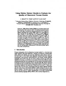
In this section we will introduce our application example which is used for illustration purposes and experiments later on. Our model represents a small part of a processing plant (see Figure 1). Two machines process indistinguishable items in non-deterministic time intervals. The characteristic of these time intervals is known and described by a continuous probability distribution. In our setting we assume that registering the times at which items leave the two machines is not possible or feasible. The streams of items processed by each machine are merged and then pass through a quality tester. This tester determines whether an item meets the required quality criteria and records the time of each test and the test result. The test itself is modeled as not consuming any time. A excerpt of such a protocol is shown in Figure 2. It contains

Processing Machine 0

Tester

Lorem ipsum dolor sit amet, consectetur adipisicing elit, sed do eiusmod tempor incididunt ut labore et dolore magna aliqua. Ut enim ad minim veniam, quis nostrud exercitation ullamco laboris nisi ut aliquip ex ea commodo consequat.

Processing Machine 1

Trace Output

Figure 1: Schematic of application example … 4514.6491648 Ok 4550.9830388 Ok 4631.0414747 Ok 4688.7225311 Ok 4754.8440860 Defect 4860.3753751 Ok 4875.6575781 Ok 4996.1659433 Ok 5015.3372168 Defect 5113.7655749 Ok …

Figure 2: Excerpt from quality tester output time stamps and the test result obtained (Ok or Def ect). Under normal operating conditions, it suffices to detect and remove items that fail to meet the company’s quality standards. But when an abnormally high number of defective items is detected, it is necessary to find the cause of this problem. The first step here will be to determine whether there is a correlation between the origin of an item and the defect probability. However, at the time that the incident is reported, the only information available is the quality test protocol. So the goal of this work is to answer the question: Is it possible to accurately determine the source (machine 0 or 1) of the items tested based only on the known system parameters (model layout, probability distributions) and the trace recorded by the automated tester? The next section will show that the example problem can be described as a Hidden non-Markovian Model.

3. 3.1

STATE OF THE ART Hidden Markov Models

Hidden Markov Models have long been the standard in modeling and analyzing systems with non-observable properties [12]. At its core, an HMM is a Discrete-Time Markov Chain (DTMC) [2]. After each step of the DTMC, the system state reached with that step causes the emission of a symbol from a known alphabet with a known probability. During analysis, the DTMC being simulated and the sequence of emitted symbols is known, but the actual internal system state is not. Efficient algorithms exist for HMMs to determine the probability of a trace (a sequence of output

symbols) [12] which is called evaluation. The decoding problem is the one relevant in this publication, where the goal is to determine the most likely sequence of internal states visited in order to create a given trace. The Viterbi algorithm [13] solves this problem efficiently for HMM. However, since their internal model is a DTMC, Hidden Markov Models are based on a discrete time step size. When used to approximate continuous time, HMMs can only model systems with exponentially distributed firing times. This is not suitable for many real life applications, where processes start and end time-dependent. In our example the intervals between the items coming from the two processing machines are normally distributed.

3.2

• non-regenerative: The age of transitions need not be reset after any transition has fired, the transitions can age independently of each other. • emit-all: All (not just some) transitions emit symbols when they fire • any number of transitions from one state to another may exist The definition of HnMMs with these variations allows for the accurate definition of our problem in terms of an HnMM. Figure 3 shows the HnMM representing our production line example using a non-Markovian SPN as hidden model. The tester has only one state, but there are two transitions that can fire, which each represent the arrival of an item from one of the sources. The intervals between the items coming from machine 0 are normally disributed with a mean of 150 seconds and a standard deviation of 25. The intervals between the items coming from machine 1 are also normally disributed with a mean of 120 seconds and a standard deviation of 20. Both transitions have a race age memory policy (RA), meaning that they do not race each other, but that they age and fire independently of the other transition’s behavior. The firing of each of the transitions emits a symbol, representing the result of the quality test Ok or Def ect. The probability of the symbols emitted by one transition sums up to one, meaning that every firing emits a symbol. Defining our problem in terms of an HnMM allows to solve it using the recently-developed general solver for HnMMs based on the Proxel method.

The Proxel Method

RA

Machine 1

Machine 0

N(120, 20)

Ok p1

Hidden non-Markovian Models

HnMMs were specifically developed in order to overcome the limitations of HMMs [9]. In an HnMM, the internal model can be any discrete stochastic system. Here we are using a kind of non-Markovian stochastic Petri net (SPN), which contains elements of some of the most common extensions to the original Petri net paradigm [1]. For HnMMs, the marking of this non-Markovian SPN is not observable during analysis. Furthermore, in HnMMs the state transitions and not the target states emit the symbols. Thus, symbols can be emitted at any point in time and allow for a more realistic modelling. Variations of HnMM with varying complexity of the solution algorithms were identified and formalized in [10]. To solve our application model, the following configuration of HnMM will be used:

3.3

RA

Defect 1-p1

N(150, 25)

Ok p0

Defect 1-p0

Figure 3: The tester model as an HnMM

The Proxel method is a state space-based simulation method to compute transient solutions for discrete stochastic systems [8, 11]. It relies on a user-definable discrete time step and computes the probability of all possible single state changes (and the case that no change happens at all) during a time step. The target states along with their probabilities are stored as so-called Proxels. To account for aging (i.e. non-Markovian) transitions, the Proxels contain supplementary variables that keep track of the ages of all active and all race-age transitions. For each Proxel created, the algorithm iteratively computes all successors for each time step. This results in a tree of Proxels where all Proxels having the same distance from the tree root belong to the same time step and all leaf Proxels represent the possible states being reached at the end of the simulation. The method introduces a computation error through the discretization of time, but the error can be controlled by reducing the time step size (which will in turn increase the computational effort required). Due to the introduction of supplementary variables [6], a state space explosion can occur, rendering the simulation of bigger models infeasible. When simulating HnMMs, the state-space explosion is somewhat limited compared to a general Proxel simulation of the same model. The reason is that the simulation of HnMMs inherently shrinks the feasible state space whenever symbol emissions occur. When a symbol emission is detected, only those successor Proxels that represent a state transition emitting this symbol need to be considered. Other general state-space reduction techniques may also be applicable [4, 7], but were not considered for this work. Proxel-based simulation deterministically explores all possible developments of the system in discrete time steps. It is therefore very well-suited to analyze HnMMs, since each path from the Proxel tree root to a leaf represents a possible state sequence of the underlying simulation model. The probability computed for the leaf is the probability of the whole path leading to that leaf. In [9] the applicability of Proxels to evaluating and decoding HnMM was shown. In this paper we will concentrate on the practical applicability to the decoding problem and necessary adaptions to make it practically feasible.

4.

COMBINING HNMM AND PROXELS

In this section we detail the application of Proxels to decoding of HnMM, meaning to determine likely system be-

havior that generated a given system output.

4.1

Adaption of Proxels to Decode HnMMs

Proxel-based simulation explores all possible future developments of a system within a discrete time step. It determines all possible follow-up states and the firing probability of the corresponding state transitions. Then the Proxels of the next time step are created and recursively the next generation determined. When applying Proxels to HnMM we need to only follow the future developments of the system, which could have produced the given output symbol sequence. Therefore, any Proxel that could not have produced the given output sequence, or would result in a different one, can be deleted and need not be further examined. This reduces the number of Proxels per time step and over the course of the simulation, reducing the overall computational effort. In detail the given output trace has the following effects: Through the trace of output symbols, the times at which state changes have to happen are known in advance. Thus, when a symbol has been emitted, the probability to stay in a give state is always zero (since a state change is known to have happened). When analyzing a HnMM where every state transition results in a symbol emission, when the given trace does not contain a symbol for the given time stamp, the probability to change the state is zero, since it is known that no symbol has been emitted and thus no state transition could have happened. However, in most Proxel implementations the path that produced a given Proxel was not stored, but only the current configuration, enabling a joining of Proxels with the same state and age in one time step. For decoding purposes we need to know the generating path, or at least a representation of the relevant properties of the generating path. This in turn increases the state space of the model significantly, since it permits the joining of Proxels with the same state and age that have a different generating path. The computation of the probability of a follow-up Proxel also needs to be adjusted slightly. While the standard Proxel method computed absolute probabilities of each Proxel, the solution algorithm for HnMMs requires the computation of conditional probabilities, i.e. the probabilities of a state change to happen under the condition that the corresponding symbol in the trace has been emitted at the given time. Therefore a state change probability needs to be multiplied by the probability of emitting the given trace symbol. The resulting Proxel simulation of an HnMM is a pruned Proxel tree that only contains state changes that can have happened to create the given trace. Each path from the root to a leaf represents a sequence of state changes that would have created the known trace, and the probability of the leaf Proxel storing the probability of that path. Hence, the pruned Proxel tree contains the information necessary to solve the HnMM and determine the most probable sequence of state changes along with the times of the state changes that would have created the trace.

4.2

Implementation Issues

Most modifications to the Proxel algorithm are straightforward to implement. But one property of the HnMM simulation requires special attention: through the modified computation of state transitions, the probabilities of individual Proxels can become very small, often even smaller than can

be represented by the IEEE 754 double type (≈ 10−300 ). Thus, an underflow occurs and most if not all probabilities will simply be set to zero, making the results useless. To solve this problem we resorted to logarithmic probabilities, the common solution for HMM analysis algorithms [5], where this problem also occurs. The probability is not stored directly, but only the logarithm of the probability. When using logarithmic probabilities, multiplication operations are replaced by a simple addition of the logarithms. The sum of two logarithmic probability values values log(a) and log(b) with a ≤ b (without loss of generality) is computed using the Kingsbury-Rayner formula: log(a + b) = log(b) + log(1 + elog(a)−log(b) ) Using this formula, a and b do not have to be computed explicitly, avoiding the possibility that their values may be to small to be represented. Since a ≤ b, the difference log(a) − log(b) will never be positive and raising e to that power will never overflow. The power may underflow if a  b and thus compute the power to be zero, but in this case the equation will evaluate to log(b), which is indeed the correct result within the limit of rounding errors. Using logarithmic values has the advantage that little overhead occurs when handling the values, but that the underflow of double precision is avoided. Multiplying probabilities generates no overhead, adding probabilities requires the additional computation of a power and a logarithm.

4.3

Adaption to Application Example

In order to make this general approach feasible for real world-application, it is necessary to adapt the computer program to the specific application case. A general Proxel HnMM solution algorithm is possible, and has been implemented in [9], but the performance is not satisfactory. When applying the general algorithm to the problem stated in Section 2, we faced memory overflows and computation times in the order of hours to analyze even short traces. The main problem is that a complete solution to the HnMM decoding problem needs to compute and store all possible generating paths along with their probabilities. That makes it impossible to merge Proxels that represent the same system state at the same time but have different histories. The resulting state space explosion could not be handled using the generic Proxel data structure. However, we found a way to reduce the state space by reducing the information needed from the generating paths. The output of our general Proxel HnMM solution algorithm is the list of all feasible generating paths along with their probability. But due to the huge number of possible generating paths (in our example, most item may have come from either machine, and thus for a sequence of n items, up to 2n different generating paths exist), obtaining the whole set of paths is usually not the desired result. Instead, the desired result is usually either the most likely path (or the m most likely paths), or some aggregate measure on all feasible paths. In our application example of the two item sources feeding one quality tester, the exact sequence of items coming from each tester is not relevant to determine who has produced more defective products. One only needs to know the amount of defective and working products produced by each machine. To retrace that, we do not need to store the generating path for each Proxel, but only the correspond-

5.

In this section we will demonstrate the results of our Proxel-based HnMM analysis and then test the behavior of the algorithm performance and results under varying conditions, such as increased trace length, increasing variation in the model distributions and even deviation of generating system from the analysis model. To test our approach, we used the simulation software AnyLogic [3] to model our system with a defect probability of 10% for items processed by machine 0, and 5% for items from machine 1. The model was then simulated with AnyLogic’s discrete event simulator to create a trace by recording the test results at the tester along with the test time stamps. To be able to validate our algorithm, the number of defective items produced by machines 0 and 1 was also stored, albeit separately. The comparison criterion we used in most cases is the relative result error (relErr). It is defined as the difference between actual defect frequency (realDF ) of a source and the detected average defect probability (guessDP ) of the source, divided again by the defect frequency (1). Where the actual defect frequency is the number of defects produced by one machine divided by the total number of items produced by that machine (2). The detected defect probability is the estimated number of defects for one machine divided by the estimated total number of items produced by the machine (3). =

realDF0

=

guessDP0

=

|realDF0 − guessDP0 | realDF0 realD0 realP0 guessD0 guessP0

0.1 0.08

(1) (2) (3)

The HnMM model used as input for the analysis algorithm was the one shown in Figure 3. When analyzing the trace we assume not to know which of the sources had the higher defect percentage, instead we assume the same failure probability of 5% for both machines. Therefore when more than 5% of the complete production are tested as defects, at least one of the sources must produce a higher defect percentage. The trace produced using AnyLogic was then fed into our Proxel HnMM solver to compute the likely numbers of defects produced by either machine. The HnMM solver

0.06 0.04 0.02 0 27

30

33

36

39

42

45

48

51

54

57

60

63

66

69

72

75

78

81

84

Number of Defective Items Machine 0

Machine 1

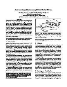
Figure 4: Probability histogram of defective items produced by either machine for a single trace. computes the probabilities for all possible numbers of defects produced by machine 0, which automatically determines the number of defective items produced by machine 1.

5.1

EXPERIMENTS

relErr0

0.12

Probability

ing aggregate number of defective items produced by one of the machines along that path (since the total number of defects is known through the trace and the number of defective items from the other machine is just the difference of these two values). This not only reduces the memory consumption of a single Proxel, but also enables joining Proxels with different generating paths that produced the same number of defects from one source. Only through this specific adaption is it possible to perform the analysis with reasonable computational effort and memory consumption. When faced with another specific application, different aggregation strategies will be needed to be make the algorithm feasible. However, usually only certain properties of the system behavior are of interest to answer a specific question, such as length or number of machine downtimes, but not the complete failure protocol. Thus, aggregation is not only necessary, but often actually desirable.

Example Analysis Result

A typical simulation result is shown in Figure 4. The histogram shows the probability distributions of the number of defects produced by machine 0 (more to the right) and machine 1 (more to the left). The two histograms are mirror images of each other. The total number of defects D is known and therefore the probability of having x defective items processed by machine 0 implies the same probability for having D − x defective items produced by machine 1. P (D0 = x) = P (D1 = D − x) This result is not trivial to obtain from the trace, since it is the essence of all possible system development paths leading to this trace, which were detected in the Proxel-based simulation. It also shows that the attribution of a defective item to one source is not unambiguous. If an item is detected about 120 seconds after the last one coming from machine 1 and about 150 seconds after the last one from machine 0, then the item could have been processed by either machine with about the same probability. This is however not an algorithmic problem, but the exact determination of the source is simply not possible based on the given data. However, our algorithm has the ability to pursue both possibilities and evaluate them independently. In the example trace analyzed, the actual number of defects produced by machine 0 was 71 and machine 1 produced 40 defects. The histogram shows that machine 0 produced more defective items than machine 1 in absolute numbers. Assuming that machine 0 produced about 40% of the items tested in total (which can be derived from the probability distributions of the model), the defect probability for items coming from machine 0 is about twice as large compared to machine 1. We can therefore state that our algorithm accurately detected the source of the unusual high number of defective items in the tested case. Our algorithm does not return a definite number of defective items produced by either machine, but a probability distribution of possible numbers. The actual likely number of defective items produced by each machine can be derived by computing the mean value of the distribution shown in the histogram in Figure 4. These numbers can then be compared to the actual number of defective items produced by that simulation run. To further evaluate our approach, four major research questions are of interest

0,14

Computed Defect Probability

Relative Error of Defect Probability

0.6 0.5 0.4 0.3 0.2 0.1

0,12 0,1 0,08 0,06 0,04 0,02 0 0

20000

40000

60000

0 0

10

20

30

40

50

2. Does the relative difference between our simulation result and the actual number of defective items produced by a machine converge when the trace length increases? 3. Does the algorithm still produce accurate results when the model creating the trace (or the trace collected at a real system) is not identical to the model used in the HnMM solver in terms of distribution characteristics? 4. How well does the algorithm scale with increasing trace length?

5.2

Influence of Randomness

The first question is of interest because it enables us to verify whether our algorithm is indeed correct. For a correctly developed and implemented algorithm, the percentage of incorrect classifications should decrease when the influence of randomness to the model is decreased. If the standard deviations of the two machines processing times grow, then the two machines become less and less distinguishable and thus the simulation result should be close to a random guess. If, on the other hand, the standard deviations are decreased, the two processing intervals become better distinguishable (since their mean values differ). For the extreme case of a standard deviation of zero, the normal distributions would degenerate to zero-width Dirac impulses, and the system would become completely deterministic, making the matching of symbol emissions to source machines a trivial task (unless two symbol emissions happen at exactly the same time). To test the convergence behavior under varying standard deviations, we varied the model shown in Figure 3 and created traces for each of these variations. The model’s two distributions’ standard deviations were varied between 5 and 50, but both standard deviations were always set to the same value. For each trace, our HnMM solver was fed with the trace and the corresponding standard deviation. It computed the overall defect probability of both machines. This number was then compared to the actual relative frequency of defective items that occurred during trace creation. Figure 5 shows the resulting relative error between the computed defect probabilities and the recorded relative de-

120000

140000

160000

180000

200000

Machine 1

Figure 6: Convergence behavior of defect probability of a single trace with increasing trace length Relative Error of Defect Probability

1. Does the relative difference between our simulation result and the actual number of defective items produced converge to zero when the standard deviations of the two normal distributions for the processing times are reduced?

100000

Machine 0

Standard Deviation of the Model's Normal Distributions

Figure 5: Convergence behavior of result error under reduction of the distributions’ standard deviation.

80000

Trace Length (s)

60

0,3 0,25 0,2 0,15 0,1 0,05 0 0

20000

40000

60000

80000

100000

120000

140000

160000

180000

200000

Trace Length (s) Trace 1

Trace 2

Trace 3

Trace 4

Trace 5

Figure 7: Convergence behavior of relative result error of multiple traces with increasing trace length

fect frequencies. The results are as expected: for high standard deviations, the accuracy is close to 0.5, as bad as a random guess would be. For standard deviations approaching zero, the accuracy increases remarkably and the error converges to zero. Since the algorithm reacts to the reduction in model variance as expected, we have another indicator that our approach produces valuable and correct results for the given example.

5.3

Influence of Trace Length

The second set of experiments was conducted to test the limits of our algorithm, i.e. to investigate whether the result accuracy increases along with the amount of information available. For this experiment, very long traces (about 3,000 symbols, 200,000 seconds of model time) were created with the usual method. They were then analyzed with our HnMM solver and intermediate results were extracted every 10,000 seconds model time. The results were then compared to the relative defect frequencies to yield the relative error of the machines’ computed item defect probability. Figure 6 shows the results for one example trace in terms of the estimated defect probabilities of both machines. With increasing trace length, the defect probabilities converge to a value close to the actual model defect probabilites used to produce the traces: machine 0 has 0.1 defect probability and machine 1 0.05. Figure 7 shows the development of the relative error for machine 0 and for five different traces with increasing length. For short traces, the accuracy of the results varies somewhat erratically, but converges to a constant value with increasing trace length. It does, however, not converge to zero. Thus, giving the algorithm more information by increasing the trace length makes the result accuracy more predictable, but does not actually increase it.

0.7

180 160 140

0.5

CPU Time (s)

Relative Error of Result

0.6

0.4 0.3 0.2

120 100 80 60 40

0.1

20 0

0 0

20

40

60

80

100

0

120

500

1000

1500

2000

2500

3000

Trace Length (#Symbols)

Range of the Added Uniform Noise

Figure 8: Result accuracy with increasing noise in the recorded output trace

Figure 9: Increase of computation time with growing trace length

The likely reason is that the trace data is itself ambiguous. Sometimes a symbol emission can be attributed to either of the machines with similar probability, making both possibilities equally likely. The actual source of the item can no longer be extracted from the data thus limiting the overall result accuracy. In very short traces, the occurrence (or absence) of a single ambiguity has a big impact on the result accuracy and accounts for the erratic changes. For longer traces, the impact of a single ambiguous situation on the result accuracy becomes smaller and smaller, making the accuracy more stable. However, since increasing the trace length also causes the introduction of new ambiguities, some uncertainty will always be part of the results, no matter how long the input trace is. Therefore, collecting an increasing amount of information is not necessary to gain more accuracy, but we need a certain minimum trace length to produce useful results. In our example about 1500 symbols, corresponding to 100,000 seconds of model time, seem sufficient to reach the maximum possible result accuracy.

be expected. This suggests that our method is quite robust against differences of the actual system parameters and the assumed model parameters. In our example application it still produces useful results even if these differ within a reasonable range.

5.4

Influence of Noise

The question of whether the algorithm is still able to compute accurate results when the model used to create the trace differs from the one fed into the HnMM solver is highly relevant for many practical applications. Here, the traces are recordings of output from real system, whereas the model for the HnMM solver is just an idealization and thus simplification of that system. An inability to compute meaningful results in the presence of these discrepancies would render the algorithm useless for practical applications. In practice the real system never exactly corresponds to an idealized model specification, there are always deviations. To test the algorithm’s robustness against model discrepancies, we created a trace for our model using the usual model parameters. We then introduced noise into the trace by adding a uniformly distributed random number to the time stamp of each test result. We varied the range of that uniform distribution from 0 to almost 100 seconds. The Proxel-based analysis algorithm still used the idealized model shown in Figure 3. Figure 8 shows the test results in terms of relative error of the detected defect probability. The result error does not increase significantly up to a maximum value of 30 seconds for the random increment, which is considerable compared to the mean values of 120 and 150 seconds of the two sources’ inter-arrival times. Up to a maximum value of 80 seconds, the relative error increases only moderately. When the data becomes too noisy, the results are no longer useful, as can

5.5

Computation Time

Testing an algorithm’s computation time behavior is necessary to assess its practicability in day-to-day operations. High computation times may require different computing environments (e.g. clusters instead of a single machine), and a disadvantageous increase of computation time with increased trace length may limit the trace length that the algorithm can sensibly process. To analyze the behavior of our algorithm, we simulated our original model on a single CPU core and measured the CPU time used to simulate the model up to certain points in model time. The results are shown in Figure 9. Since the algorithm is based on the Proxel method, its computation time behavior similarly increases exponentially with increasing simulation time (trace length), but with a low initial slope. For a trace containing symbol emissions for a time interval of 10000s (about 3 hours), the computation time amounted to about three seconds. Even for a trace of 200,000 seconds (about 55 hours), the computation took less than three minutes, which is still reasonable. And as previous experiments showed that an increased trace length does not translate to higher result accuracy, the exponential growth of computation time does not seems to be a relevant problem in the analysis of this model. It should be noted, however, that the model is a very simple one and more complex models may substantially increase the computational complexity.

5.6

Discussion of Experiments

In the experiment section we tried to validate our method and test its performance behavior under growing input size. We first illustrated that our method returns a set of possible system behaviors, that could have produced the recorded trace. These can be combined to form probability distributions of certain system characteristics. This is significantly more information than to only compute the most likely system behavior that generates the given trace. One can even estimate the reliability of the result by observing the overlap in the resulting probability distributions of different values of system characteristics. The first set of experiments confirmed our expectation

that our simulation results vary less with decreasing standard deviation (and thus decreasing randomness) in the input model. Reducing the standard deviation and thereby the variation, makes the symbol origin in the trace less ambiguous and thereby increases the accuracy of our analysis. This strengthens our confidence in the correctness of our algorithm. The second set of experiments tested the impact of input size on the simulation result. The error in the simulation result converged to a certain value with increasing input trace length. This value is however not zero for larger model variance, since there will always be ambiguities in the symbol trace interpretation. However, with increasing trace length the results became more reliable and we were able to determine the cause of the unusual system behavior. Another experiment tested the robustness of the method under the influence of noise, which can also be regarded as a deviation of the model from the real system. We introduced a discrepancy between the model and the system by adding random noise of increasing strength to the signal trace. Our method seems quite robust in the tested example case, still producing correct results even with considerable noise added to the signal stream. This increases the applicability to real processes, since there the system specification might only be known roughly or might even be subject to certain fluctuations, rendering a model that exactly represents the real system an impossibility. The performance experiments showed an exponential increase in computation time with growing trace length, which matches the behavior of the original Proxel method. However, the exponent is not high and the resulting computational effort still within minutes and therefore acceptable for practical applications. Furthermore does an increased input size not automatically result in less error in the result, eliminating the need for further increases in input trace length.

6.

CONCLUSION

In this paper we introduced an approach to reconstruct unobservable behavior of discrete stochastic systems from recorded output protocols. The challenge in the field of discrete stochastic systems is, that the output itself is ambiguous and does not seem to contain enough information to retrace the behavior of the complex system that produced the output. We presented a method that uses a Hidden non-Markovian Model to represent the partially-observable system and its output, and Proxel-based simulation to analyze a recorded output symbol trace. Using this combination it is to our knowledge possible for the first time to reconstruct discrete stochastic system behavior solely based on time-stamped output protocols. We illustrated the method using a small production line example where items flows from two sources are merged and result in one quality test protocol. The source of an item is not recorded in the test protocol and cannot easily be determined in hindsight. Our method determined possible item defect probabilities and their probability distribution. We were thereby able to determine which input stream was the cause of an unusually high error percentage as long as the streams were by themselves sufficiently different in regard to distribution parameters. Our experiments showed that the method could successfully extract the relevant information from the recorded production output at a reasonable expense

of computation time. The presented approach is limited to models with a relatively small state space, since Proxel-based simulation is only applicable to small models. The actual maximum feasible model size depends on the model structure and parameters. As a rule of thumb, the discrete state space should not contain more than ten states and the age vector should at no time need to track the age of more than four transitions. However, elaborate protocol data could enable the analysis of larger models by rendering many possible system developments impossible and thus reducing the problem state space. We believe that this approach can be very helpful in the industry today. Many production lines for example do not incorporate internal sensors due to the large effort needed to record and analyze a complex and consistent production protocol. However, often the production output is monitored in order to detect deviations from predefined production parameters. Using our method we can use this output to retrace the source of a problem from historical data and at no extra expense of sensory equipment. The approach could also be used to monitor production lines by external sensor equipment and then retrace the causes of problems, if the production parameters under normal operating conditions are known. The approach can also be applied to an arbitrary, not completely observable discrete stochastic system. The actual course of a disease of a certain patient can be retraced by analyzing the protocol of his body temperature, blood pressure or various other measurements, if a comprehensive model of the disease is available. One could also determine the likely source of a traffic jam on a major road by analyzing the traffic flows already recorded at different points along the road and its intersections. A future task is to test our approach using real data protocols and determine the maximum complexity of systems that can still be analyzed using our approach. Alternatively we can also incorporate multiple output data protocols, recorded at different points in the process to gain insight into more complex systems. Hidden non-Markovian Models can also deal with noisy input data, due to the stochastic nature of the output symbols. The effect of noise on the analysis result also needs to be tested in the future. A long term goal is to be able to determine actual system parameters, such as failure intervals and distribution parameters, for partially observable systems based only on recorded production output data. This could be used to build simulation models of systems where the parameters are unknown and cannot be determined by direct measurements.

7.

REFERENCES

[1] A. Bobbio, A. Puliafito, M. Telek, and K. S. Trivedi. Recent developments in non-markovian stochastic petri nets. Journal of Systems Circuits and Computers, 8(1):119–158, 1998. [2] G. Bolch, S. Greiner, H. de Meer, and K. S. Trivedi. Queuing Networks and Markov Chains. John Wiley & Sons, New York, 1998. [3] A. Borshchev and A. Filippov. From system dynamics and discrete event to practical agent based modeling: Reasons, techniques, tools. In Proceedings of 22nd International Conference of the System Dynamics Society, Oxford, England, July 2004.

[4] E. de Souza e Silva and P. M. Ochoa. State space exploration in markov models. SIGMETRICS Perform. Eval. Rev., 20:152–166, June 1992. [5] G. A. Fink. Markov Models for Pattern Recognition, chapter 7, page 121. Springer Berlin Heidelberg, 2008. [6] R. German. Transient analysis of deterministic and stochastic petri nets by the method of supplementary variables. In Proceedings of the 3rd International Workshop on Modeling, Analysis, and Simulation of Computer and Telecommunication Systems (MASCOTS 95), pages 394–398. IEEE Computer Society, 1995. [7] B. R. Haverkort. In search of probability mass: Probabilistic evaluation of high-level specified markov models. The Computer Journal, 38(7):521–529, 1995. [8] G. Horton. A new paradigm for the numerical simulation of stochastic petri nets with general firing times. In European Simulation Symposium, Dresden, Germany, October 2002. SCS European Publishing House. [9] C. Krull and G. Horton. The effect of rare events on the evaluation and decoding of hidden non-markovian models. In Proceedings of the 7th International Workshop on Rare Event Simulation (RESIM 2008), Rennes, France, September 2008. [10] C. Krull and G. Horton. Hidden non-markovian models: Formalization and solution approaches. In Proceedings of 6th Vienna International Conference on Mathematical Modelling, Vienna, Austria, February 2009. [11] S. Lazarova-Molnar. The Proxel-Based Method: Formalisation, Analysis and Applications. PhD thesis, Otto-von-Guericke Universit¨ at Magdeburg, 2005. [12] L. R. Rabiner. A tutorial on hidden markov models and selected applications in speech recognition. Proceedings of the IEEE, 77(2):257–286, February 1989. [13] A. H. Viterbi. Error bounds for convolutional codes and an asymptotically optimal decoding algorithm. IEEE Transactions on Information Theory, IT-13:260–269, April 1967.