Using Hierarchical Spatial Data Structures for Hierarchical ... - CiteSeerX

Timpf, S. and A. U. Frank (1997). Using hierarchical spatial data structures for hierarchical spatial reasoning. Spatial Information Theory - A Theoretical Basis for GIS (International Conference COSIT'97). S. C. Hirtle and A. U. Frank. Berlin-Heidelberg, SpringerVerlag. Lecture Notes in Computer Science 1329: 69-83.

Using Hierarchical Spatial Data Structures for Hierarchical Spatial Reasoning Sabine Timpf and Andrew U. Frank Dept. of Geoinformation Technical University Vienna {timpf, frank}@geoinfo.tuwien.ac.at

Abstract This paper gives a definition of Hierarchical Spatial Reasoning, which computes increasingly better results in a hierarchical fashion and stops the computation when a result is achieved which is ‘good enough’. This is different from standard hierarchical algorithms, which use hierarchical data structures to improve efficiency in computing the correct result. An algorithm on hierarchical spatial data structure explores all details where such exist. An hierarchical reasoning algorithm stops processing if additional detail does not effectively contribute to the result and is thus more efficient. Hierarchical spatial data structures, especially quadtrees, are used in many implementations of GIS and have proved their efficiency. Operations on hierarchical spatial data structures are effective to compute spatial relations. They can be used for hierarchical spatial reasoning. A formal definition of hierarchical spatial reasoning requires • a coarsening function c, which produces a series of less detailed representations from a most detailed data set, • a function of interest f which is applicable to these representations, and • a function f’ which computes for each representation the quality of the result. The computation starts with the least detailed representation and continues till a result with sufficient quality is found. This is demonstrated with a simplified example, based on a raster computation for area computation and overlap. Examples from the literature demonstrate that the same hierarchical aggregation and similar coarsening functions can be used for a wide variety of spatial reasoning tasks.

1 Introduction Effective spatial reasoning systems must use hierarchical approaches, similar to methods humans typically use (Stevens and Coupe 1978). Recently, the term ‘hierarchical spatial reasoning’ has been used (Car and Frank 1994a; Jones and Luo 1994; Whigham 1993) and several examples explore such ideas (Abler, Adams, and Gould 1971; Dutton 1993; Noronha 1988; Hirtle and Jonides 1985; Fotheringam 1992; Goodchild 1990; Bemmelen van et al. 1993). Golledge has included ‘hierarchical reasoning’ in a recent list of the most important open questions in spatial reasoning (Golledge 1992). Cohn has discussed coarser and finer representations (Cohn 1995) and Papadias and Glasgow (Glasgow and Papadias 1992) have extended symbolic projections to hierarchical situations. Different levels of spatial resolution are typical for topographic maps and map series of varying scale can be seen as hierarchies (Timpf and Frank 1995). Whigham extends

Timpf, S. and A. U. Frank (1997). Using hierarchical spatial data structures for hierarchical spatial reasoning. Spatial Information Theory - A Theoretical Basis for GIS (International Conference COSIT'97). S. C. Hirtle and A. U. Frank. Berlin-Heidelberg, SpringerVerlag. Lecture Notes in Computer Science 1329: 69-83.

the hierarchical structure to both space and time in which events happen (Whigham 1993). These efforts have provided some points in this wide and admittedly very important field of hierarchical reasoning, but a general framework for hierarchical spatial reasoning and a definition for it are still missing. This hierarchical approach is imitating approaches humans use when performing spatial reasoning tasks: an appropriate level of detail is selected (e.g., the scale of the map used) and the result computed. The quality of the result is then assessed and compared with the requirements of the process. If the quality of the result is sufficient to make the decision, then the process stops; if it is not yet sufficient, the next level of more detailed data (e.g., maps of larger scale) is consulted. Hierarchical reasoning computes approximation with error bounds. It is the application of a non-hierarchical spatial reasoning algorithm to a series of increasingly finer (higher resolution) representations of the same situation, giving a series of improving approximations of reality. For each application of the algorithm not only the value is computed, but also bounds on the errors, which allows to determine when the approximation is good enough for the given task. This is more efficient as computing is not wasted to refine a result which is good enough. Spatial reasoning is used here to denote any deduction of information from a representation of a spatial situation. It includes the simple calculation of spatial predicates, e.g. the area of a region, and spatial relations, i.e. the intersection of two areas, used here as running example, but also all operations of map algebra (Tomlin 1983a; Tomlin 1983b), symbolic spatial reasoning, etc. (Freksa 1992; Freksa 1991) (Cohn et al., to appear) and more complex tasks like planning of routes, shortest path (Bemmelen van et al. 1993), allocation of resources, viewsheds (Fisher 1996) etc. Hierarchical spatial reasoning applies hierarchical reasoning to spatial situations. It concentrates the elaboration of the function of interest to areas where more detail is needed and areas where a decision can be made on a less detailed level are excluded. Hierarchical data structures (Samet 1989a; Samet 1989b) have been developed and optimized for particular spatial algorithms. It was found that the quadtree data structure with a nearly infinite number of variants is generally very useful for many different tasks and leads to efficient algorithms for spatial data with high spatial autocorrelation. This paper explores how the concept of hierarchical data structures can be extended to hierarchical processing methods exploring the hierarchy to compute increasingly better results until the quality of the result is sufficient for the decision to be made. There are also other efforts for hierarchical structures in spatial information theory, defining hierarchical divisions of curves (Ballard 1981), hierarchical triangulation (De Floriani and Puppo 1992; Puppo and Dettori 1995), and hierarchical networks (Car and Frank 1994). Timpf has shown how a spatial task is broken down hierarchically into subtasks (Timpf et al. 1992) and Voisard has formalized similar task subdivisions for a mapping system (Rigaux, Scholl, and Voisard 1993; Voisard and Schweppe 1994). This paper is structured as follows: The following section discusses hierarchies and hierarchical reasoning. Then the two examples of spatial reasoning used as running examples are introduced. Section 5 shows how traditional spatial reasoning is performed on an array and a quad tree. Then the next section gives the essence of hierarchical reasoning which is then formalized in section 7. In section 8 incremental

Timpf, S. and A. U. Frank (1997). Using hierarchical spatial data structures for hierarchical spatial reasoning. Spatial Information Theory - A Theoretical Basis for GIS (International Conference COSIT'97). S. C. Hirtle and A. U. Frank. Berlin-Heidelberg, SpringerVerlag. Lecture Notes in Computer Science 1329: 69-83.

processing is proposed as a further improvement. The last section presents conclusions and lists open questions regarding possible limits for the method.

2 Hierarchies are Crucial for Spatial Reasoning Space is continuous in two dimensions and can be observed from many different points of view and at different resolution. The same objects can be represented differently, depending on the purpose, indicating the point of view to take and the level of detail to be included. This is generally called ‘multiple-representation’ of spatial objects (NCGIA 1989; Buttenfield 1993; Buttenfield and Delotto 1989; Timpf 1997). The representation of a spatial object at different levels of resolution leads to hierarchical representation: more and more details are included as one descends the hierarchy. Space is often conceived as container, in which certain objects or properties are held. Containment forms a transitive relation, which leads to a hierarchy of containers (often, to be precise, a heterarchy or lattice (Greasley 1990)). Many operations naturally generalize along such container hierarchies: highest peak, area, population count, topological relations, shortest path (Bemmelen van et al. 1993), viewshed (Fisher 1996) etc. Aggregation along a container hierarchy respects spatial neighborhood and one is tempted to extend the idea of Klein (Klein 1872) to classify geometric properties by invariance to form a new class - perhaps called spatial - for all operations which remain invariant under spatial aggregation and the rules for hierarchical reasoning as defined here. Data base research has typically considered space as a single continuum. This is theoretically sound and sufficient, but leaves out the potential for shortcuts given through the hierarchical organization of the data by humans. Difficulties are observed in practical applications: The cadastral database of Austria contains all parcel boundaries of Austria; in principle one can deduce the country boundary processing every boundary parcels contribution to the boundary, but this requires much processing and is most likely also inappropriate in the level of accuracy achieved. Hierarchical spatial reasoning uses the level of detail appropriate for the task. This is an economic principle: a task is solved with the least amount of effort. Effort is reduced by selecting a level of detail which is sufficient for the task, but not finer. Effort is further reduced by excluding areas from detailed inspection which do not contain detailed relevant data. Working through more details does not contribute to the solution comparable with the cost of the additional computation: computing better solutions costs increasingly more, but contributes decreasingly less value to the solution. The quality of a result can be measured on different scales, not only precision. The relevant aspect depends on the decision to make. It is assumed here that the quality of the result is assessed on an ordered scale (in the sense of Stevens (Stevens 1946)), and an assessment if a given result is ‘good enough’ can be made. The specifics of the quality measure is not important - in the example simple bounds for maximal error are used.

3 Hierarchical Spatial Reasoning Follows Patterns of Human Cognition There is evidence that hierarchical spatial reasoning approaches are used in human spatial mental reasoning. Several experiments revealed hierarchical organization of

Timpf, S. and A. U. Frank (1997). Using hierarchical spatial data structures for hierarchical spatial reasoning. Spatial Information Theory - A Theoretical Basis for GIS (International Conference COSIT'97). S. C. Hirtle and A. U. Frank. Berlin-Heidelberg, SpringerVerlag. Lecture Notes in Computer Science 1329: 69-83.

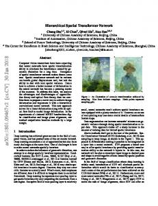
spatial data and processes (Stevens and Coupe 1978; Tversky 1993; Hirtle and Jonides 1985; Hirtle 1995). We assume, that imposing hierarchies on unstructured data helps humans to reason about this data. This seems to be especially true for spatial data. Observing typical errors in human spatial inferences reveals that mental reasoning processes follow hierarchical patterns (Figure 1). A Reno

A County California

Nevada

B County B

San Diego

1) A in A County 2) B in B County 3) A County North of B County -> A North of B

1) San Diego in California 2) Reno in Nevada 3) Nevada East of California -> Reno East of San Diego

Fig. 1. Example for correct and erroneous reasoning using hierarchies (according to (Stevens and Coupe 1978))

Human behavior follows nearly always this pattern and deviations are ridiculed: the engineer, who computes the diameter of a pencil to 15 places after the decimal point; the accountant, who declares the gross income of a company as $13,435,342,677.42 etc., all demonstrate some basic incomprehension of the limits to measurements of real world objects. The lay person marvels at the precise measurements possible today, when the length of the year can be determined down to very small fractions of a second, or the distance from Europe to the USA measured with an accuracy better than one centimeter. Standard measurement practice by lay persons seems to yield 1/1000, professionals achieve 1 PPM and specialists can push precision even further (to 10-12). In most practical circumstances, such precision is not warranted. But in all cases values measured have an error associated - no measurement is absolutely precise. Hierarchical reasoning, as intuitively applied by humans, works because the interactions of processes in the world are clustered around some characteristic level of detail: the size of everyday small objects, buildings, are two typical levels of detail, where many interactions occur. For each task an appropriate level of detail is known from experience (Fraser 1981). Informally, one can observe many examples of this general behavior in everyday situations: while driving a car, one does not worry about its parts; while planning a building subdivision, the plants in the future gardens are not considered. But on a higher level, the properties of the parts are represented in a generalized form and used directly for decision-making. Spatial reasoning is infinitely complex, because the spatial world is infinitely complex. Hierarchical structuring of this complexity is crucial to reduce the spatial reasoning tasks to manageable levels. Hierarchical structures have been introduced by

humans to arrive at a manageable complexity; it is imperative that these methods are integrated into data processing methods. This paper gives an abstract description, independent of particular applications, which can be implemented and then used generally.

4 Running Example: Area Calculation and Intersection Test As a running example, two simple tasks, one a spatial calculation, the other a test for a spatial relation, are selected. They are applied to regions represented in a regular tessellation (raster) but the extension to irregular tessellations (so-called ‘vector data structures’) should not cause problems (De Floriani and Puppo 1992; Frank 1987). One of the simplest spatial calculation is the calculation of the size of the area (Figure 2). The standard method for computing the area in an array (or generally raster structure) is to count the resels inside the area. As a typical test for a spatial relation, the check if two areas intersect is used (Figure 2). Two regions are intersecting if there is any resel inside both of them. For this we have to check for each corresponding pair of resels if two are both inside the respective region, which is to say that this resel is inside both.

Area = 6

= Intersection Fig. 2. Area size calculation and intersection test

5 Computation on Array and Quadtree The prototypical representation for a regular tessellation - especially of a square tessellation - is a regular array. Numerous methods for more compact data structures are known, e.g. run length encoding and various quad tree data structures. 5 . 1 Array Representing regions as array of resels fills much storage space and results in slow processing, as a large number of resels must be inspected. The effort for the computation is linear in the number of resels and therefore in the size of the array, independent of how much of the space is filled with objects of interest, how much is background etc. 5 . 2 Quadtree Spatial data is often highly spatially correlated - this means that the probability that similar values are clustered is very high. This spatial autocorrelation is exploited in quadtrees to encode larger areas with the same value as a single unit (Samet 1989b). Recursively, a quadtree is either a leaf with a uniform value or it is a tree with four

quadtrees. It is customary to interpret a quadtree structure as a representation of space, in which the leaf nodes are resels in a square array (Figure 3). Resels of higher level represent four times the area of the resel one level lower. The values of the resels represent a property of the area (encoded typically as a binary value).

Fig. 3. Example of a Quadtree

To compute the area, the quadtree is traversed and the leaves which are inside (black) are summed, taking into account that leaves higher up in the hierarchy represent larger areas. To decide if two regions, both represented as quadtrees with the same spatial orientation intersect, both quad trees must be traversed in parallel and decided for each node if an intersection is possible or not. The computation using a quadtree data structure produces the same result as the corresponding full resel array, only faster. The result is always completely accurate, and all details of the data which contribute to the result must be inspected. Processing of the quadtree follows most often a depth first pattern, which leads to simpler algorithm.

6 The Principle of Hierarchical Reasoning Hierarchical reasoning is based on the economic principle to use the least detailed representation sufficient to answer a question. All data is inherently imprecise, but decisions do not require perfect information, but information which is sufficiently precise. Computing more detail is a waste as it does not contribute to the solution. Hierarchical reasoning implies data structures where multiple representations with increasing level of detail and therefore increasing precision are stored. The hierarchical reasoning progresses from the least detailed representation to more detailed ones and for each the result is computed and an error assessment made. If the error of the current result is smaller than the required quality for the result, the process stops. Hierarchical reasoning requires a method to derive less detailed representations from the most detailed one. This is shown in the next section for the simple case of regular raster, but can be extended to irregular triangulations (De Floriani and Puppo 1992) and other irregular subdivisions of space. 6 . 1 Coarsening Function to Derive Less Detailed Representations From a given array of resels at maximal resolution a sequence of coarser representations are constructed by grouping together four resels and giving them a new value: ‘inside’ if all four smaller resels are inside, ‘outside’ if they are all outside. For the mixed case, we can either employ a majority rule (3 resels inside give ‘inside’ for the aggregate, 3 resels outside give ‘outside’ for the aggregate), but

to decide on the split case (2 inside, 2 outside) is difficult. Fisher discusses regular spacing, mean, maximum and minimum and maximum deviation from mean as methods to coarsen a landscape (Fisher 1996). The solution selected here is an ‘all’ rule: only all inside or all outside cases are recorded as inside or outside in the coarser representation and all mixed cases marked as such. Resels can then have 3 values, inside, outside or mixed (Figure 4). Mixed resels are considered as ‘don’t know’ values and are used to assess the error in the computation (this will force a three-valued logic (Sinowjew 1968) in the computation). W

W

W

W

M

M

W

B

B

W

W

B

W

W

B

B

W

W

B

B

M

Fig. 4. Three different levels of coarseness in a regular tessellation

6 . 2 Hierarchical Computation of Area and Intersection The computation for the area and the intersection values must include also the computation for the error bounds to stop the progress of the elaboration of increasingly better values. (This is easiest achieved by defining a data type of value and error as a pair and then all computations (e.g., intersection, addition etc.) extended for these data types). For the area size black and white resels are added, but the mixed resels add only to the error estimate. The test for intersection is performed by pairwise comparison of corresponding resels. • if there is any certain overlap, the intersection test yields true; • if there is no certain overlap, but any maybe value, the intersection test yields maybe (the sum of the size of maybe resels gives a bound for the error); • if all resels are ‘no overlap’, the intersection test yields false. This is the extension of the ‘or’ operation to a three-valued logic (Sinowjew 1968).

7 Spatial Hierarchical Reasoning Spatial hierarchical reasoning assumes that the given values have a certain error and that results need only to be computed at a level of certainty appropriate for the task at hand. Both are often only implied assumptions and need to be made explicit for the formulation of hierarchical reasoning algorithms. The estimate of the error in the values given is associated with the coarseness level of their representation and must be introduced quantitatively. The tolerated error in the result must be given in the same measurements. It is assumed to be directly related to the spatial resolution of the resels.

7 . 1 Conditions for Spatial Hierarchical Reasoning To apply spatial hierarchical reasoning, the following is necessary: • an algorithm f to work on a representation ri of the facts at a given level of detail (in our case a resel array of a given resolution) producing a value vi ; • an algorithm f’ to work on the representation ri and producing an estimate of the error ei on the result of applying f to the representation ri , yielding vi ; • a filter c to produce a sequence of representations ri , such that ri-1 is coarser than ri 1. The computation at one level of detail must yield a result which is compatible with the result of the next level with more detail and, by transitive extension, eventually compatible with the true result. The approximations must monotonically improve towards the correct result. This imposes a number of conditions on the coarsening operation and the spatial reasoning operation. 7 . 2 Formal Conditions Given a sequence of representations of the same situation with increasingly more detail: r1, r2 K ri K rm where r1 is the coarsest and rm is the most detailed representation. The coarsening operation c produces ri-1 from ri : ri-1 = c (ri ) The operation of interest f applied to each element of this sequence of ri produces a sequence of values vi and with the corresponding error estimation function f’ a sequence of error estimates ei . v1, v2 K vm with vi = f (r i ) e1, e2 K em with ei = f’ (ri ) Conversion Towards Correct Result. The computations must converge towards the correct result. This requires that the error bounds get more and more restraining. This means that the sequence e1, e2 K em must monotonically decrease, i.e. ei ≥ e i+1. This gives the condition f’(c(ri )) ≥ f’(ri ) for the functions f’ and the coarsening function c (because ei = f’r and ei+1 = f’ri+1 = f’(c(ri )) ). This is the case for the coarsening function on arrays and the computation of error bounds as the sum of the ‘mixed’ resel: the coarsening operation produces a larger and larger area of mixed resel (if one of the four resels is mixed, the result of the coarsening is mixed).

1

Observe the ordering of the representations, which proceeds from the coarsest to the finest: r0 is the coarsest representation, ri is the finest; therefore ri-1 = c(ri ).

Non-Contradiction of More Detailed Values. The value reported by the calculation with a more detailed representation must not contradict the value achieved with a less detailed representation. For Boolean values resulting from the intersection calculation, once a value of true or false is achieved, all computations with more detail must produce the same value. Only for a value of vi = maybe, the value vi+1 can be either true or false. For the calculation of area, the value vi is the sum of the inside resels. The total area can vary between vi and vi + ei , and vi + ei /2 is usually the most probable value. The interval resulting from a more detailed computation with representation rj (with j>i) [vj , vj +ej ] must be inside the interval resulting from the detail level ri , which is [vi , vi +ei ]. Termination. The computation of the values in the sequence progresses till a value vi is found, for which the error bound ei is smaller than the error which can be tolerated for the decision to be made. No further computation is necessary. The sequence of error values decreases monotonically (see subsection on conversion) and reaches ultimately 0 for the most detailed representation, which is assumed to have no error.

8 Optimization: Incremental Spatial Reasoning Spatial reasoning as broadly defined above is computing the value for each representation from scratch, repeating for all areas where there is no additional detail, the same calculation for each level, achieving the same results. This is clearly inefficient and can be improved using an incremental approach: instead of recomputing the value for the representation ri from scratch, the value obtained from ri-1 is used and only the increments Dvi and Dei are computed and added to vi-1 and ei1.

M

M W

W W

M B

W

W

W B

B

W

Fig. 5. Arrows for the computation, show repetition

To compute the increment, only areas which have details must be inspected; in the representation used here, only mixed resels must be visited. Calculating the area, only the mixed resels add to the area count and decrease the error level. When calculating the intersection and the overall result is maybe , only resels which yielded maybe must be inspected on the more detailed level to see if a true or false result can be obtained.

The same incremental concept is applied to the data structure resulting in hierarchical incremental data structures (Figure 5), where a finer level of detail contains only the increment in detail and does not repeat the representation of the areas, where the coarser and finer representation agree. Such data structures have, in the best case, the same size as non-hierarchical ones and give all the advantages of multiple representations. A regular quadtree can be transformed into a structure which gives the nodes for each level (in left to right order) - this is the result of single breadth first traversal (and can be done in linear time in the number of nodes). The incremental quadtree can be represented as a list of levels, each level as a list of the nodes (coded as above as I, O or M). This transformation can be reversed, as all details are preserved (the transformation is loss-less). The number of nodes remains the same and storage is very compact as no pointers are stored (this is closely related to the linearized, pointerless quadtree (Samet 1989a, p. 55) resulting from a depth-first traversal).

9 Conclusions and Open Questions Humans apply hierarchical concepts to spatial situations. Langacker - a prominent cognitive linguist - states “Hierarchy is crucial to human cognition” (Langacker 1987). Hierarchy is the major conceptual tool to structure the infinite levels of detail in our spatial environment and it is widely used by humans for spatial inferences ((Hirtle and Jonides 1985), (Hirtle 1995), (Stevens and Coupe 1978), (Tversky 1993)). Structuring space with a spatial inclusion (container) hierarchy is most effective if combined with a reasoning strategy which computes values only as precise as necessary. Results are deduced at the coarsest level of detail to reduce the amount of facts to be considered. Areas, for which it is possible to quickly exclude that they contribute to the solution, are considered settled and not further explored. Quadtrees are a well known, efficient method to structure spatial data hierarchically. The standard algorithms applied to them compute efficiently the correct result with minimal effort. Spatial hierarchical reasoning allows further improvements: a computation is only pushed to produce a result with sufficient precision for the decision at hand. Spatial hierarchical reasoning proceeds in steps of increasing resolution and produces increasingly better approximations to the correct result, till an approximation is found which is ‘good enough’ (as judged from the task at hand). In real-time applications, the same method can be used to compute a series of increasingly better approximations to fulfill stringent requirements on response: it is sometimes more important to have a first approximation quickly, then to wait till the correct result becomes available too late. Spatial hierarchical reasoning is thus the combination of • a data structure which provides increasingly more detail and computes an error bound on the approximation, and • an algorithm which computes the desired value and an error bound for it (this is generally recommended for spatial algorithms, but seldom done for most computation in a geographic information system, where input data are always somewhat erroneous). Spatial hierarchical reasoning can be optimized if the data structure and the algorithm permit incremental processing. Incremental spatial hierarchical reasoning

proceeds to compute a result and then computes a series of increments, which improve the previous result. 9 . 1 Results Hierarchical spatial reasoning is more efficient than computing the most precise answer, as computation is stopped when a result of sufficient quality is achieved. Using incremental methods, it is (nearly) as efficient to compute the best result than traditional methods, except that it produces intermediate useful values. The methods presented here can be extended to other spatial reasoning tasks. Examples from the literature show many operations from spatial analysis which operate in this context: even shortest path (Bemmelen van et al. 1993) and viewshed (Fisher 1996) can be applied to representations with less detail. Both operations produced approximate results. 9 . 2 Open questions It seems that a large number of spatial analysis operations can be brought into this framework. Klein classified spatial relations in topological, metrical etc. based on the group of transformation they are invariant under (Klein 1872). One could extend this notion to call operations spatial if they are invariant (in the special sense with error bounds) to spatial coarsening. Open remain a number of specific questions regarding the limits of the use of this strategy: Hierarchical Map Algebra. A large part of practical spatial reasoning is described with the concept of map algebra. Implementations are widely available. How much of these operations can be carried over into this framework? In principle all of them, because any operation can be applied to the representation expanded as an array of resels (of the given level), but more efficient solutions should be possible, using the results from research in efficient algorithm in quadtrees (Mark and Lauzon 1985). The difficult task is to determine the corresponding functions to compute errors for spatial analysis functions. Hierarchical Reasoning on Irregular Tessellations The discussion here was in terms of a regular tessellation, but applies in principle equally to irregular. Efforts to construct hierarchies of irregular tessellations have been started (De Floriani and Puppo 1992; Puppo and Dettori 1995; Bruegger and Egenhofer 1989; Bruegger and Frank 1990). Hierarchical Reasoning for Line or Point-based Spatial Problems Car has studied hierarchical reasoning for a hierarchically structured network and used the shortest path problem as her leading example (Car 1996). She proposed a definition of hierarchical reasoning which applies to linear problems and must be generalized to coincide with the one given here.

References Abler, R., J.S. Adams, and P. Gould. 1971. Spatial Organization - The Geographer's View of the World. Englewood Cliffs, N.J., USA: Prentice Hall.

Ballard, D.H. 1981. Strip Trees: A Hierarchical Representation for Curves. ACM Comm. 24 (5): 310-321. Bemmelen van, et al. 1993. Vector vs. Raster-based Algorithms for Cross Country Movement Planning. Proceedings of AUTO-CARTO 11, at Minneapolis, USA. Bruegger, B.P., and M.J. Egenhofer. 1989. Hierarchies over Topological Cells for Databases. Proceedings of GIS/LIS '89, at Orlando, FL. Bruegger, B.P., and A.U. Frank. 1990. Hierarchical extensions of topological data structures (P301.2). Proceedings of FIG XIX Congress, June 10 - 19, at Helsinki, Finland. Buttenfield, B.P. 1993. Multiple Representations - Closing Report. Buffalo: State University of New York at Buffalo. Buttenfield, B.P., and J.S. Delotto. 1989. Multiple Representations: Report on the Specialist Meeting - Initiative 3: NCGIA, Santa Barbara, CA. Car, A. 1996. Hierarchical Spatial Reasoning: Theoretical Consideration and its Application to Modeling Wayfinding. Ph.D. Thesis, GeoInfo Series Vol 10, Department of Geoinformation, Technical University Vienna. Car, A., and A.U. Frank. 1994a. General Principles of Hierarchical Spatial Reasoning - The Case of Wayfinding. Proceedings of SDH'94, at Edinburgh, Scotland. Car, A., and A.U. Frank. 1994b. Modeling a Hierarchy of Space Applied to Large Road Networks. In IGIS'94: Geographic Information Systems. Proceedings of International Workshop on Advanced Research in GIS, in Ascona, Switzerland, edited by J. Nievergelt, et al. Berlin: Springer-Verlag. Cohn, A.G. 1995. A Hierarchical Representation of Qualitative Shape Based on Connection and Convexity. In Spatial Information Theory-A Theoretical Basis for GIS, edited by A. U. Frank and W. Kuhn. Berlin: Springer-Verlag. Cohn, A.G., et al. to appear. Representing and Reasoning with Qualitative Spatial Relations about Regions, Dordrecht, The Netherlands: Kluwer Academic Publishers. De Floriani, L., and E. Puppo. 1992. A Hierarchical Triangle-Based Model for Terrain Description. In Theories and Methods of Spatio-Temporal Reasoning in Geographic Space, edited by A. U. Frank, I. Campari and U. Formentini. Berlin: Springer-Verlag. Dutton, G. 1993. Scale change via hierarchical coarsening: cartographic properties of Quaternary Triangular Meshes. Proceedings of 16th Int. Cartographic Conference, at Koeln, Germany. Fisher, P. 1996. Propagating effects of database generalization on the viewshed. Transactions in GIS 1 (2): 69-81. Fotheringam, A.S. 1992. Encoding Spatial Information: The Evidence for Hierarchical Processing. In Theories and Methods of Spatio-Temporal Reasoning in Geographic Space, edited by A. U. Frank, I. Campari and U. Formentini. Berlin: Springer-Verlag. Frank, A.U. 1987. Overlay Processing in Spatial Information Systems. Proceedings of AUTO-CARTO 8, at Baltimore, MD. Fraser, J.T., ed. 1981. The Voices of Time. Second Edition. Amherst: The University of Massachusetts Press. Freksa, C. 1991. Qualitative Spatial Reasoning. In Cognitive and Linguistic Aspects of Geographic Space, edited by D. M. Mark and A. U. Frank. Dordrecht, The Netherlands: Kluwer Academic Press. Freksa, C. 1992. Using Orientation Information for Qualitative Spatial Reasoning. In Theories and Methods of Spatio-Temporal Reasoning in Geographic Space, edited by A. U. Frank, I. Campari and U. Formentini. HeidelbergBerlin: Springer-Verlag.

Glasgow, J.I., and D. Papadias. 1992. Computational imagery. Cognitive Science 16 (3): 355-394. Golledge, R.G. 1992. Do People Understand Spatial Concepts: The Case of First-Order Primitives. In Theories and Methods of Spatio-Temporal Reasoning in Geographic Space, edited by A. U. Frank, I. Campari and U. Formentini. Heidelberg-Berlin: Springer Verlag. Goodchild, M.F., and Y. Shiren. 1990. A Hierarchical Data Structure for Global Geographic Information Systems. Proceedings of 4th International Symposium on Spatial Data Handling, at Zurich, Switzerland. Greasley, I. 1990. Partially Ordered Sets and Lattices: Correct Models of Spatial Relations for Land Information Systems. MSc. Thesis, University of Maine, Orono. Hirtle, S.C., and J. Jonides. 1985. Evidence of Hierarchies in Cognitive Maps. Memory & Cognition 13 (3): 208-217. Hirtle, S.C. 1995. “Representational Structures for Cognitive Space: Trees, Ordered Trees and Semi-Lattices.” In Spatial Information Theory-A Theoretical Basis for GIS, ed. Frank, A.U., and Kuhn, W. 327-340. 988. Berlin-Heidelberg-New York: Springer-Verlag. Jones, C.B., and L.Q. Luo. 1994. Hierarchies and Objects in Deductive Spatial Databases. Proceedings of Sixth International Symposium on Spatial Data Handling, SDH'94, at Edinburgh, Scotland. Klein, F. 1872. Comparative Considerations about Recent Geometric Investigations (in German). Erlangen, Verlag Andreas Deichert. Langacker, R.W. 1987. Foundations of Cognitive Grammar. Vol. 1 Theoretical Prerequisites. Stanford, CA: Stanford University Press. Mark, D.M., and J.P. Lauzon. 1985. The space efficiency of quadtrees: an empirical examination including the effects of 2-dimensional run-encoding. GeoProcessing 2: 367-383. NCGIA. 1989. The Research Plan of the National Center for Geographic Information and Analysis. IJGIS 3(2): 117 - 136. Noronha, V.T. 1988. A Survey of Hierarchical Partitioning Methods for vector Images. Proceedings of Third International Symposium on Spatial Data Handling, at Sydney, Australia. Puppo, E., and G. Dettori. 1995. Towards a Formal Model for Multiresolution Spatial Maps. In Advances in Spatial Databases (Proceedings SSD'95), edited by Egenhofer, M. J. and J. R. Herring. Heidelberg-Berlin: Springer-Verlag. Rigaux, P., M. Scholl, and A. Voisard. 1993. A Map Editing Kernel Implementation: Application to Multiple Scale Display. In Spatial Information Theory: Theoretical Basis for GIS, edited by A. U. Frank and I. Campari. HeidelbergBerlin: Springer Verlag. Samet, H. 1989a. Applications of Spatial Data Structures. Computer Graphics, Image Processing and GIS. Reading, MA: Addison-Wesley. Samet, H. 1989b. The Design and Analysis of Spatial Data Structures. Reading, MA: Addison-Wesley. Sinowjew, A.A. 1968. Über mehrwertige Logik. Berlin: Deutscher Verlag der Wissenschaften. Stevens, A. , and P. Coupe. 1978. Distortions in judged spatial relations. Cognitive. Psychology 10: 422-437. Timpf, S. 1997. A multi-scale data structure for cartographic objects. In Geographic Information Research: Bridging the Atlantic, edited by M. Craglia and H. Couclelis. London: Taylor & Francis, pp. 224-234 Timpf, S., and A. U. Frank. 1995. A Multi-Scale DAG for Cartographic Objects. Proceedings of ACSM/ASPRS, at Charlotte, N.C. Timpf, S., G.S. Volta, D.W. Pollock, and M.J. Egenhofer. 1992. A Conceptual Model of Wayfinding Using Multiple Levels of Abstractions. In Theories and

Methods of Spatio-Temporal Reasoning in Geographic Space, edited by A. U. Frank, I. Campari and U. Formentini. Heidelberg-Berlin: Springer-Verlag. Tomlin, C.D. 1983a. Digital Cartographic Modeling Techniques in Environmental Planning. Ph.D. Thesis, Yale University. Tomlin, C.D. 1983b. A Map Algebra. Proceedings of Harvard Computer Graphics Conference, at Cambridge, Mass. Tversky, B. 1993. Cognitive Maps, Cognitive Collages, and Spatial Mental Model. In Spatial Information Theory: Theoretical Basis for GIS, edited by A. U. Frank and I. Campari. Heidelberg-Berlin: Springer-Verlag. Voisard, A., and H. Schweppe. 1994. A Multilayer Approach to the Open GIS Design Problem. Proceedings of 2nd ACM-GIS Workshop, at New York. Whigham, P. 1993. Hierarchies of Space and Time. In Spatial Information Theory: Theoretical Basis for GIS, edited by A. U. Frank and I. Campari. HeidelbergBerlin: Springer-Verlag.