If you do not have Analysis Tool Pak installed on your computer, use this set of ... Data Analysis â Performs the regression of the S&P 500 and Dow Chemical ...
Journal of Business Case Studies – November/December 2010
Volume 6, Number 6
Using Hyperlinks To Create A Lecture On Calculating Beta And The Beta Coefficient For Dow Chemical Company Nakita Harper, Norfolk State University, USA Keshawna Jordan, Norfolk State University, USA Carl B. McGowan, Jr., Norfolk State University, USA Benjamin J. Revello, Norfolk State University, USA
ABSTRACT In this paper, we show hyperlinked Power Point lecture slides that show how to calculate the beta coefficient for Dow Chemical Company using the S&P 500 as the market index. This paper shows how to collect data for both Dow Chemical and for the S&P 500 Stock Index, how to calculate monthly returns, and how to run a regression to calculate the beta. The data for both Dow Chemical and for the S&P 500, fifty-one month end prices including dividends, are down loaded from Yahoo! Finance and loaded into an Excel worksheet which is used to calculate monthly returns. The fifty monthly returns are regressed with the S&P Index return as the independent variable and the Dow returns as the dependent variable. The returns are graphed to check that the analyst ran the regression properly. Keywords: beta coefficient, Power Point, CAPM, market model
MODERN PORTFOLIO THEORY
M
arkowitz (1952) develops the basis for modern portfolio theory by describing the relationship between risk and return for efficient portfolios on the efficient frontier. The efficient frontier is the set of all portfolios that have the highest rate of return for a given level of risk or the lowest level of risk for a given rate of return1. When the efficient frontier is combined with the utility preference function for the investor, a specific portfolio can be defined which will optimize utility for the selected investor. The optimal portfolio will provide the investor with the highest possible return for the given level of risk selected for the investor. Conversely, the optimal portfolio will provide the lowest possible risk for the given return level selected by the investor. Tobin (1958) adds a risk-free asset to the investment universe which allows investors to separate the investment decision from the investing decision2. Each investor selects a mix of the risk-free asset and the market portfolio based on the individual investor’s utility preference for risk and return. However, the capital market line, as it is called, only applies to efficiently diversified portfolios. However, not all portfolios are efficient, such as an individual stock. Total risk can be decomposed into two components, systematic risk and unsystematic risk. Unsystematic risk is firm specific and can be diversified while systematic risk is market driven and cannot be diversified. Sharpe (1961) develops an asset pricing model for securities based on market risk only. Systematic risk is estimated for a single asset using the regression line of the linear regression between a market index and the returns for an individual stock. The slope of this regression is the beta coefficient for the stock and is the measure of systematic risk. The regression is usually performed with five years of monthly data or sixty monthly observations. 1 2
This concept is called to Dominance Principle. This is called the Separation Theorem.
77
Journal of Business Case Studies – November/December 2010
Volume 6, Number 6
Beta is estimated using the market model in which the return for the stock is equal to the x-axis intercept, αi, plus the firm’s beta, βi, times the return on the market, Rm, plus the error term, ε. Ri = αi + βi (Rm) + ε Koller, Goedhart, and Wessels (2005, pp. 313-314) suggest that regressions for individual companies be run with sixty monthly observations against a value-weighted index such as the S&P 500. The regression demonstrated in this paper is performed with the return for the S&P 500 as the independent variable, that is, the market index, and the return for Dow Chemical is the dependent variable. Monthly returns are calculated for the S&P 500 and Dow Chemical for five years which yields sixty monthly returns. The focus of this paper is to demonstrate a Hyperlinked, Power Point Presentation to perform the process of down loading the data needed to calculate the Characteristic Line for Dow Chemical Company using the S&P 500 Index as the independent variable3. We show how to download the data, how to manipulate the data to calculate the monthly returns, how to regress the data, and how to graph the results for comparison purposes. THE POWER POINT PRESENTATION There are nine separate Power Point files and three Excel files hyperlinked to the main file. Appendix A provides a list and description of the twelve files. There are a total of fify Power Point Slides. The master Power Point file hyperlinked to the other files and is called Regression Main. To execute this program, highlight the “Regression Main” icon and double, left click. This will call up the file which will then be run as a slide show by clicking “Slide Show” and “From the Beginning.” The remaining PPT files are executed by clicking on each set of commands such as “Obtain S&P 500 Data.” The Power Point files are available from the corresponding author. Power Point Files – Hyperlinked 1.
Obtain S&P 500 Data – download the S&P 500 monthly, dividend adjusted prices. a. This file takes one to Yahoo! Finance where one clicks on “S&P 500”. b. Next, one clicks on “Historical Prices.” c. Set the “Start Date” and the “End Date” and indicate that you want to download “monthly” data. Click on “Get Prices.” The data will appear in spreadsheet format. d. Scroll to the bottom of the spreadsheet and click on “Download to Spreadsheet.” e. Select “Open with” Microsoft Office Excel (default)” to download the data into an Excel spreadsheet. Click “OK” at the bottom of the command window. f. Click on the Microsoft Office Button in the upper left-had corner and select “Save As” to save the file. Type in the File Name such as “S&P500”, select the file type Excel Worksheet, and click the “Save” button in the lower left-had corner of the command window.
2.
Obtain Company Data - download the Dow Chemical monthly, dividend adjusted prices. a. This file takes one to Yahoo! Finance where one enters the company “Ticker Symbol” in the space before the “Get Quotes.” Command. b. Next, one clicks on “Historical Prices.” c. Set the “Start Date” and the “End Date” and indicate that you want to download “monthly” data. Click on “Get Prices.” The data will appear in spreadsheet format. d. Scroll to the bottom of the spreadsheet and click on “Download to Spreadsheet.” e. Select “Open with” Microsoft Office Excel (default)” to download the data into an Excel spreadsheet. Click “OK” at the bottom of the command window. f. Click on the Microsoft Office Button in the upper left-had corner and select “Save As” to save the file. Type in the File Name such as “Dow Chemical”, select the file type Excel Worksheet, and click the “Save” button in the lower left-had corner of the command window.
3
Benninga (2008, 95-101) shows how to down load data from the internet to compute beta.
78
Journal of Business Case Studies – November/December 2010
Volume 6, Number 6
3.
Arrange Data – Combines the S&P 500 and Dow Chemical returns. a. Click on the Microsoft Office Button and select “Open” and find the “Regression PP” folder and select “Save As” to save a new Excel workbook named “DOW Regression”. b. Click on the Microsoft Office Button and select “Open” find the “Regression PP” Folder and select the “S&P 500” workbook. Click “Open”. c. Copy the “S&P 500” date in Cells A1:A62 to the new workbook “DOW Regression” beginning in Cell A1. d. Copy the “S&P 500” data in Cells G1 to G62 to the new workbook “DOW Regression” beginning in Cell B1. e. Click on the Microsoft Office Button and select “Open” find the “Regression PP” Folder and select the “DOW” workbook. Click “Open”. f. Copy the “DOW” date in Cells A1:A62 to the new workbook “DOW Regression” beginning in Cell C1. g. Copy the “DOW” data in Cells G1 to G62 to the new workbook “DOW Regression” beginning in Cell D1. h. Compare the dates in Cells A2:A62 and C2:C62 to ensure that they are the same. i. Highlight Cells D1:D62 and select “Cut” with Ctrl-x. Click on Cell C1 and paste the “DOW” data by selecting Cntrl-v. j. Rename Column B “Adj Close S&P” and Column C “Adj Close Dow”. k. Click on the Microsoft Office Button and select “Save” and find the “DOW Regression PP” file to save the data working file.
4.
Arithmetic Return – Computes the monthly arithmetic returns for the S&P 500 and Dow Chemical. a. Label Cell D1 “ROR S&P” and Cell E1 “ROR Dow.” b. Type = (B2-B3)/B3 in Cell D2. c. Highlight Cell D2, align the cursor to the bottom right corner of Cell D2 until the small cross icon appears. Left click and hold and slide the Icon to the right into Cell E3 and then release. This copies the return calculation for S&P 500 one column to the right (Cell E2) which will calculate the return for Dow. d. Highlight both Cell D2 and Cell E2, align the cursor to the bottom right corner of Cell E2 until the small cross icon appears. Left click and hold and slide the Icon down to the bottom of the data column, and then release. This copies the return calculation for S&P 500 one column to the right (Cell E2) which will calculate the return for Dow. e. Format the cells with six decimals by highlighting the data from B1 to E60 and click on “Format”, “Format Cells”, “Number”, and use “Up Arrow” to “6.” Click “OK.”
5.
Load Analysis Tool Pak – Shows how to load the Analysis Tool Pak on the computer. a. If you do not have Analysis Tool Pak installed on your computer, use this set of commands. b. Left click the “Microsoft Office Button” and select “Excel Options” c. Select “Add-Ins.” d. Highlight “Analysis Tool Pak” from the add-ins menu. e. Click OK. f. Click “Go.”
6.
Data Analysis – Performs the regression of the S&P 500 and Dow Chemical returns. a. Left click the “Data” tab and you should see “Data Analysis” to the right. Left click “Data Analysis.” b. Highlight “Regression from the Analysis Tools menu and click “OK.” c. Set the input ranges. Set the “Input Y range” from E2:E61 and the “Input X range” from D2:D61. The X range is the S&P data and the Y range is the Dow Chemical data. The X range is the independent variable and the Y range is the dependent variable. Default is to output the results in a new spreadsheet. d. Click “OK.”
79
Journal of Business Case Studies – November/December 2010
Volume 6, Number 6
7.
Results a. The output table for the regression results will be in a separate spreadsheet. The results include the adjusted R2, the F-statistic, and the regression coefficients. b. For this regression, the adjusted R2 for the regression is 0.3282, the F-statistic is 29.82, and the regression slope coefficient is 1.13 and is statistically significant at the 0.0000 level.
8.
Graph – Graphs the S&P 500 and Dow Chemical returns. A common mistake is to reverse the X range and the Y range. Graphing the data and getting the same results mitigates this problem. a. Highlight Cell D1:E61. b. Click on the “Insert” tab c. Click on the “Scatter” tab. d. Select the “Scatter Plot” option. e. Highlight one of the Data Points and then Right Click. f. Select “Add Trendline” from the menu. g. Select “Display Equation on chart” from the “Format Trendline” menu. h. Close the “Format Trendline” menu. i. Click and drag the equation from within the graph to the right side. j. The slope and the intercept terms should be the same as calculated in the regression. Otherwise, you reversed the variables in the regression or the graph. k. To format the axis, highlight the horizontal axis with a right click., Click “Format Axis” from the menu. Click “Number” and change 6 to 2 for the numbers on the axis. Repeat this process for the Y axis.
Everyone should have the same answers. If not, check the input data for similarity throughout the entire process. Typical errors involve students downloading different time periods or different a number of observations. Table 1 shows the results for the regression of the S&P 500 returns and the Dow Chemical returns. The regression coefficient, beta, is 1.1333 and the intercept, alpha, is -0.0077, and the Adjusted R2 is 0.3282. The same statistics appear on the Graph in Figure 1, indicating that the regression and the graph are correct. Table 1: Dow Chemical Regression Results Regression Statistics Multiple R R Square Adjusted R Square Standard Error Observations
0.5827 0.3396 0.3282 0.0592 60
ANOVA Regression Residual Total
df 1 58 59
SS 0.1046 0.2034 0.3080
MS 0.1046 0.0035
F 29.82
Significance F 0.0000
Intercept X Variable 1
Coefficients -0.0077 1.1333
Standard Error 0.0077 0.2075
t Stat -1.0020 5.4609
P-value 0.3205 0.0000
Lower 95% -0.0230 0.7179
80
Upper 95% 0.0077 1.5487
Journal of Business Case Studies – November/December 2010
Volume 6, Number 6
Figure 1: ROR DOW
0.15 0.10
Dow Chemical Returns
0.05
-0.20
-0.15
-0.10
0.00 -0.05 0.00 -0.05
y = 1.1333x - 0.0077 0.05
0.10 ROR DOW
-0.10
Linear (ROR DOW)
-0.15 -0.20 -0.25 -0.30 -0.35 S&P 500 Returns
SUMMARY AND CONCLUSIONS This paper provides a Power Point file that can be used to teach students to how to collect data for the S&P 500 and Dow Chemical that can be used to calculate sixty monthly returns. These returns are used in the market model regression to compute the beta coefficient for Dow Chemical. This paper provides Power Point slides to demonstrate how to graph the data both to see the relationship between the returns for the S&P 500 and Dow Chemical and to function as a check to assure that the regression was run properly. AUTHOR INFORMATION Carl B. McGowan, Jr., PhD, CFA is a Professor of Finance at Norfolk State University. Dr. McGowan has a BA in International Relations (Syracuse), an MBA in Finance (Eastern Michigan), and a PhD in Business Administration (Finance) from Michigan State. From 2003 to 2004, he held the RHB Bank Distinguished Chair in Finance at the Universiti Kebangsaan Malaysia and has taught in Cost Rica, Malaysia, Moscow, Saudi Arabia, and The UAE. Professor McGowan has published in numerous journals including Applied Financial Economics, Decision Science, Financial Practice and Education, The Financial Review, International Business and Economics Research Journal, The International Review of Financial Analysis, The Journal of Applied Business Research, The Journal of Diversity Management, The Journal of Real Estate Research, Managerial Finance, Managing Global Transitions, The Southwestern Economic Review, and Urban Studies. KeShawna Sherree Jordan is a recent college graduate from Norfolk State University in July of 2010, with a Bachelor of Science Degree in Business-Finance. During her college experience, she has become a dedicated member to the Finance and Banking Club, as well as participated with different volunteer programs. She is currently working with the City of Chesapeake in the Public Utilities Department. In the near future, KeShawna would like to pursue her Master's Degree in Business Administration and to soon work for a major finance corporation or the Government assisting in its Finance/Accounting department. 81
Journal of Business Case Studies – November/December 2010
Volume 6, Number 6
REFERENCES 1. 2. 3. 4. 5.
Benninga, Simon. Financial Modeling, Third Edition, The MIT Press, Cambridge, 2008. Koller, Tim, Marc Goedhart, and David Wessels. Valuation: Measuring and Managing the Value of Companies, Fourth Edition, John Wiley and Sons, Inc., Hoboken, NJ, 2005. Markowitz, Harry. “Portfolio Selection,” The Journal of Finance, March 1952, pp. 77-91. Sharpe, William F. “Capital Asset Prices: A Theory of Market Equilibrium under Conditions of Risk,” Journal of Finance, September 1964, pp. 425-552. Tobin, James “Liquidity Preference as Behavior Towards Risk,” The Review of Economic Studies, February 1958, pp. 65-86.
82
Journal of Business Case Studies – November/December 2010
Volume 6, Number 6
APPENDIX A Regression PPT File
Regression Main – The master Power Point file hyperlinked to the other files. Power Point Files – Hyperlinked 1. 2. 3. 4. 5. 6. 7. 8.
Obtain S&P 500 Data – download the S&P 500 monthly, dividend adjusted prices. Obtain Company Data - download the Dow Chemical monthly, dividend adjusted prices. Arithmetic Mean – Computes the monthly arithmetic returns for the S&P 500 and Dow Chemical. Arrange Data – Combines the S&P 500 and Dow Chemical returns. Data Analysis – Performs the regression of the S&P 500 and Dow Chemical returns. Graph – Graphs the S&P 500 and Dow Chemical returns. Load Analysis ToolPak – Shows how to load the Analysis ToolPak on the computer. Results
Excel Spreadsheet Files 1. 2. 3.
S&P 500 – This file contains the S&P 500 downloaded data. Dow – This file contains the Dow Chemical downloaded data. Dow Regression – This tile combines the Dow Chemical and the S&P 500 data and is used to perform the regression and constructs the graph.
83
Journal of Business Case Studies – November/December 2010 NOTES
84
Volume 6, Number 6