Using Imperfect Advance Demand Information in Forecasting Tarkan Tan Department of Technology Management, Eindhoven University of Technology, P.O. Box 513, 5600MB Eindhoven, The Netherlands
[email protected] Abstract: In this paper we consider the demand forecasting problem of a make-to-stock system operating in a business-to-business environment where some customers provide information on their future orders, which are subject to changes in time and hence constituting imperfect advance demand information (ADI). The demand is highly volatile and non-stationary, not only because it is subject to seasonality and changing trends, but also because some individual client demands have significant influence on the total demand. In such an environment, traditional forecasting methods may result in highly inaccurate forecasts, since they are mostly developed for the total demand based only on the demand history, not making use of demand information and ignoring the effects of individual order patterns of the customers. We propose a forecasting methodology that makes use of individual ordering pattern histories of the product-customer combinations and the current build-up of orders. Moreover, we propose making use of limited judgmental updates on the statistical forecasts prior to the use of ADI. In our application at a company that produces dairy ingredients this method resulted in significant improvements in the forecasts and as a result, required safety stocks are reduced by 25% by incorporating ADI in forecasts, and we demonstrated that the reduction amounts to 37% in case judgmental updates are also utilized. Keywords: Advance Demand Information, Forecasting, Judgmental Updates
1
1
Introduction
In many business-to-business environments the demand exhibits high volatility and nonstationarity, not only because it is subject to seasonality and changing trends, but also because some individual client demands have significant influence on the total demand. Nevertheless, some customers may provide information on their future orders, which are subject to changes in time and hence constituting imperfect advance demand information (ADI). In this paper we consider the demand forecasting problem of such a make-to-stock system where we propose some forecasting methods that make use of this ADI. Our problem is motivated by a dairy products company who sells basic and specialized ingredients for the food and dairy industry worldwide and owns production locations in several countries. The orders to the company are placed either as single orders or as a call off that is part of a contract. The company operates in a make-to-stock manner and the production decision is based on forecasts. Safety stocks are kept to cover for the forecast errors. The forecast is used for several planning activities such as • Packaging- and raw material acquisition • Production planning • Financial forecasting that serves the purpose of controlling whether budgets are met • International milk allocation planning (milk distribution between various plants) • Reserving inventory space in warehouses. A more accurate forecast will improve various performance indicators such as delivery reliability, amount of inventory carried, utilization rate, financial forecast accuracy and the quantity of obsolete packaging- and raw materials. The nature of the business-to-business environment makes it possible to collect ADI from some customers, since the customers have their own production plans that are known in advance to the materialization of their orders, which is usually not the case in business-toconsumer environments. Sometimes this is to give the supplier the time to arrange transport for deliveries to other parts of the world, but it may also be the case that orders are part of contracts. The quantity sold in these contracts is split in several deliveries that take place during the term agreed in the contract. The customer calls for the quantity ordered a certain 2
lead time in advance (the demand lead time). Another reason for the customers to order in advance is to minimize the risk of unmet orders. In our application, we observed that in average 30% (even 57% for a particular product) of the orders of a month were already known by the end of the previous month, where the production lead time is approximately 1 month. This apparently creates a good opportunity to improve any forecasting method that ignores such information. In some cases the demand lead time is as long as 9 months or more. If it is known that an order that is placed in advance will be materialized without any change, this constitutes “perfect ADI”. In many cases however, previously placed orders are subject to changes in time. When the available information on future demand -or the information that can be collected and processed in rather easy and inexpensive ways particularly due to advances in information technologiesincludes impurity and uncertainty, we refer to this kind of ADI as “imperfect ADI”. In our application the orders that were placed in advance were almost never postponed or cancelled, and the changes were occurring only in forms of increased orders. We made use of this observation in our methods, but we note that similar methods can be devised for different forms of ADI. In many of such business-to-business environments, judgmental forecasts are preferred to statistical forecasting methods due to high volatility and non-stationarity of demand. Specific customer information such as a customer ceasing operations for a certain period, a capacity extension of a customer that will result in increased orders, and the like can only be collected and utilized by judgmental forecasts that are conducted by personnel that have in-depth information on individual customers, such as Area Sales Managers (ASMs). An ASM is a sales representative that visits customers for reasons such as making contracts and therefore s/he has in-depth information on individual customers. Nevertheless, such a forecast consists of forecasts on each product-customer combination (PCC) for a certain time horizon, which may be a very labor-intensive task that repeats itself every period. It is very time consuming for the ASMs to analyze all past demand data and information from the the database of the company. Because there is little time to get the data available, ASMs often make their forecasts without any additional information or help, resulting in elevated forecast inaccuracies. The methods we propose also make a limited use judgmental forecasts, benefiting from such individual information and yet decreasing the workload of the ASMs significantly. The remainder of the paper is organized as follows. In Section 2 we review the related 3
literature briefly. We discuss our problem environment further in Section 3 and we propose a forecasting methodology in Section 4. We propose some methods that can be used in demand forecasting based on imperfect ADI in Section 5. Finally, we present our conclusions and discuss possible extensions in Section 6.
2
Related Literature
Selecting a particular forecasting method is complicated. Many factors that are specific to the environment have to be taken into account. Abraham and Ledolter (1983) identify 5 parameters that influence the choice for a certain model: Degree of accuracy, forecast horizon, forecasting budget, complexity required, and availability of data. These parameters depend on the item whose demand is to be forecasted and also interact with each other. Besides the choices that have to be made for these parameters, also the forecast type has to be chosen. Chatfield (2001) classifies the forecasting methods that have been developed into three types: 1. Judgmental forecasts, based on subjective judgment, intuition, commercial knowledge and other available information 2. Univariate methods, where forecasts depend only on present and past values of the single series being forecasted, possibly added to a function of time such as linear trend 3. Multivariate methods, where forecasts of a given variable depend on values of one or more additional time series variables, which are called predictor or explanatory variables. The methods that we propose make use of time series, judgement, and information at the same time, therefore do not fit into one of these classes. Our purpose in proposing such methods is to benefit from the advantages of each of these factors, in an attempt to avoid the disadvantages of basing the forecasts on a single factor. Makridakis and Wheelwhright (1989) define 4 types of judgmental forecasting: jury of executive opinion, sales force composites, anticipatory surveys and individual subjective assessments. Field studies show this method is commonly used in business. See, for example, Winklhofer and Diamantopoulos (2002), and Klassen and Flores (2001). Bunn and Wright (1991) indicate that the reason why judgmental forecasting is favored is that planners identify 4
severe limitations in using purely statistical techniques. Most important complaint is that statistical techniques are not able to forecast one-time events. DeLurgio (1997) states that the basic assumption of forecasting is that the past patterns or behavior will continue into the future. If the pattern is broken statistics will fail and only humans are able to predict this. For these reasons we also advocate not using purely statistical techniques. On the other hand, although only humans are able to predict pattern breaks, humans are not always very good at it! Studies show humans tend to exaggerate changes in patterns, causing large forecast errors (Makridakis, 1988). Goodwin and Fildes (1999) show that judgmental forecasters also perform poor in integrating judgmental and statistical input to one forecast. It is often the case that statistical forecasts are changed when they are highly reliable and ignored when they should be used to improve the judgmental forecast. For those reasons we also advocate not using purely judgmental forecasts. Goodwin (2002) also advocates integrating judgmental and statistical forecasts by arguing that “Human judges are adaptable and can take into account one-off events, but they are inconsistent, can only take into account small amounts of data and suffer from cognitive biases. In contrasts, statistical methods are rigid, but consistent and can make optimal use of large volumes of data.” Our major contribution in this paper is integrating advance demand information -both perfect and imperfect- with a combination of judgmental and statistical forecasts. In what follows, we review the related literature on ADI briefly. ADI is mostly treated in the production/inventory context. The term “advance demand information” is coined by Hariharan and Zipkin (1995) where they show that perfect ADI improves the performance of a continuous-time inventory system in the same way as a reduction in lead-times. Gallego ¨ and Ozer (2001) show the optimality of a state-dependent order-up-to policy in a discretetime setting, where the states are formed by perfect ADI and inventory. Dellaert and Melo (2003) deal with the lot-sizing problem in a similar environment. Karaesmen et al. (2002) consider a capacitated problem under perfect ADI and stochastic lead times. They model the problem via a discrete time make-to-stock queue. We refer the reader to Karaesmen et al. (2003) for a literature survey and treatment of perfect ADI in production/inventory systems. The literature on different forms of (imperfect) ADI has been rapidly increasing in recent years. Treharne and Sox (2002) consider a problem where the demand in any given period arises from one of a finite collection of probability distributions. DeCroix and Mookerjee (1997) consider a periodic-review problem in which there is an option of purchasing demand 5
information at the beginning of each period. Van Donselaar et al. (2001) investigate the effect of sharing imperfect ADI between the installers of a project and the manufacturers, in a project-based supply chain. Thonemann (2002) elaborates further on a similar problem in which there is a single manufacturer and a number of installers. Zhu and Thonemann (2004) consider a problem that consists of a number of customers that may provide their demand forecasts. Tan et al. (2007) consider an imperfect ADI situation where information is modeled in a rather general way. In their model a portion of the prospective demands stays in the system for one or more number of periods before either being materialized as demand or leaving the system. All the above work utilize ADI in their respective settings and come up with inventory policies (in some cases optimal inventory policies) and show the benefits of imperfect ADI. We are not aware of any work that considers utilizing imperfect ADI in forecasting. To the best of our knowledge, the only work on utilizing perfect ADI in forecasting are by Thomopoulos (1980) and Abuizam and Thomopoulos (2005), where they propose making use of Bayesian updates. Nevertheless, as we discuss in Section 3 Bayesian updates have the shortcoming of dependence on distributional assumptions, as well as the updates being one-sided.
3
Advance Demand Information
In this section we present the imperfect ADI structure that we consider in this work. As introduced in Section 1, we observed this structure at a dairy products company operating in business-to-business environment. Instead of considering the whole demand on a product, we consider each product-customer combination (PCC) individually, in order to make bast use of information. These forecasts constitute the total forecast on the product once they are aggregated over all customers. While some customers never change their orders that are placed in advance, some others update their orders in time (increases in our case) and some others never provide any information prior to the materialization of demand. At the time that an order is placed, it generally cannot be determined if this order will be changed or not. Nevertheless, in some cases it is (almost) certain that this ADI is perfect, such as orders that are guaranteed by contracts. Besides, it is possible to classify some other orders as perfect ADI (i.e., current ADI is expected to be materialized as demand with no change) by analyzing the order his6
tory of that PCC. For that purpose, the individual ordering pattern histories of the PCCs should be observed and PCC profiles should be built accordingly. If a customer has never changed her previously placed orders of a product in history, it is possible to refer to the ADI obtained from her as perfect ADI, because the customer proved to provide reliable information. Similarly, if a customer has made a certain number of updates on the information she provided and the order history of that customer shows that there has never been more updates made by the customer in her demand history, then we recommend classifying this information also as perfect ADI. Naturally there is a risk of misclassifying an imperfect ADI as perfect, but especially if sufficient data on the profile of the PCC exists, this risk should not be very significant. Consequently, we propose the following classification as to the quality of information: If the number of updates a customer i has made on her ADI on product j is less than her historical maximum Mij , it is considered as imperfect ADI, otherwise it is considered as perfect ADI. Naturally, there is also a group of customers who place their orders without providing any demand information in advance. We refer to this kind of demand as “NoADI demand”. We propose some forecasting methods that make use of these patterns and the current build-up of orders. There is no standardized approach available for the use of advance demand information. Therefore this chapter will explore how advance demand information available at DMV can be used. Since the number of orders per month varies and the order sizes reveal no information about the demand volume that can be expected in the same period, it is useful to have an estimator for the number of orders that is expected in a certain month. This estimator can be generated by the statistical forecasting tool, but this will only be useful when a regular pattern can be expected in the number of orders per month. In the next section several methods will be described that estimate demand, based on imperfect ADI. The methods described will be tested on a sample of product/customer combinations to find out which one performs best. In the production/inventory models that make use of ADI in the literature, a common approach is to classify the demand into two groups: “observed” and “unobserved” demand (referring to orders placed in advance and unannounced orders, respectively), assuming that they are independent. However, such an approach would be inappropriate here. Customers that do not provide information in some periods may provide information in some other 7
periods, and customers that provide information on some certain period’s demand may further place unannounced demand at that period. Therefore, observed and unobserved demands are not generated by non-overlapping populations, and hence the independence assumption is severely violated. Moreover, such a classification would not be making the best use of information, since customer profiles would not have been used in that case. In such an environment, traditional forecasting methods may result in highly inaccurate forecasts, since they are mostly developed for the total demand based only on the demand history, not making use of demand information and ignoring the effects of individual order patterns of the customers. While there is no method available in the literature -to the best of our knowledge- that take the information on the individual order patterns of the customers into account, it is possible to make use of Bayesian updates in order to utilize advance demand information. Nevertheless, Bayesian updates have some shortcomings. In order to illustrate these shortcomings, we first refer to an example provided by Thomopoulos (1980). Suppose that at time T , knowledge of a future demand of 75 pieces for T + 4 becomes available. Assuming that the current forecast and standard deviation for this period are 100 and 25, respectively, and that the demand is normally distributed, the adjusted forecast for T + 4 becomes 102. Note that any observation will result in the forecast to be higher than that without any information. In other words, if the ADI amounts to a quantity much less than the average, Bayesian update results yet in an increased forecast and it is not possible that imperfect ADI signals a less-than-average demand using Bayesian updates. Next, we refer to an example provided by Abuizam and Thomopoulos (2005). Consider a situation where at the current time period T , the forecaster learns that there are two advance orders scheduled for T +3, with corresponding order sizes of 91 and 100, respectively. Historically, average number of orders is 5.25 and average order size is 89.01 units. Assuming that the number of orders has a Poisson distribution and given the current forecast for time T + 3 is equal to 467.33 units, the updated forecast becomes 562.69 units. Observe that, while the observed demand in the first example is relatively higher, the update in the second example is much more dramatic. This is due to different distributional assumptions of these two cases. Moreover, only the information as to the total observed demand (or total number of observed orders) is utilized in Bayesian updates, and information on the individual order patterns of PCCs is not taken into account. To summarize, the major shortcomings of Bayesian updates are 8
1. they depend on distributional assumptions, 2. the updates are one-sided, 3. customer order patterns are not taken into account.
4
Proposed Forecasting Methodology
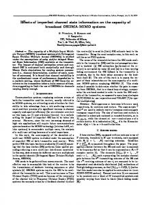
In this section we present a methodology that can be used in making forecasts in the environment that is described. This approach uses statistical forecasting, judgmental forecasting, and advance demand information to produce a final forecast for demand. The advantages of judgmental input and the strengths of statistical input can be combined by forecasting all PCC demands with the most appropriate statistical techniques and then have the ASMs view and modify only a limited number of those for the changes to the regular pattern they expect, in order to make sure that important information is not overlooked. Automatic generation of a statistical forecast reduces the chances of forecast errors due to unrecognized demand patterns. The input from ASMs can be used to forecast events that break the demand pattern. We propose making use of judgmental updates only for key PCCs (prior to the use of ADI). Depending on the business, the PCCs that represent larger production volumes, higher costs, higher risks for obsolete stock, and the like could be among the selection criteria for the key PCCs. Such limited input decreases the workload of the ASMs, while the system is still benefiting from the specific customer information for the key PCCs and controlling the level of subjectivity on the forecasts. Moreover, the reason of the updates should be recorded and followed up. When the ASMs are required to motivate and record every change they make, the proposed changes need to be well thought out. As Goodwin (2002) points out, the accuracy increases most by judgmental input when the judges are asked to motivate their changes. This also allows better feedback, because the system remembers why a forecast was altered. We refer to the demand forecast of the PCC of concern for a future period t that have been generated this way (and perhaps with the involvement of some other bodies in the organization) as the “forecast agreement”, F At . The methodology that we propose is to take this forecast as the basis and then to incorporate advance demand information with it to generate the “final forecast” of that PCC. See Figure 1 for a schematic representation of this methodology. Naturally, the statistical forecast that is updated by making use of available 9
ADI could also be considered as the basis that the ASM reviews and her judgmental changes could constitute the final forecast, depending on the reliability of the judgmental changes. A hybrid methodology that first adapts the proposed methodology and then switches to the other one (where the judgmental changes are final) as sufficient experience has been built could also be considered.
M o n th ly c y c le
S ta tis tic a l fo re c a s t
A S M in p u t
F o re c a s t a g re e m e n t
E v a lu a te a c c u ra c y
R e a l-tim e
A D I
F in a l F o re c a s t
Figure 1: Proposed Methodology
The next step is how to incorporate demand information with the forecast agreement. This depends on the available information. If no ADI is available for this PCC, the forecast agreement becomes the final forecast. If perfect ADI is available, then this information overrides the forecast agreement, since this information is made up of already placed orders and it represents (or is assumed to represent) the future demand with no uncertainty. The case of imperfect ADI is more complicated. In what follows, we propose some forecasting methods for this case.
5
Incorporating Imperfect ADI in Forecasting
In this section we propose some forecasting methods that make use of imperfect ADI for a PCC of concern. We summarize our major notation in Table 1. 1. Basic Method: Ft = max{F At , Ot }
10
Table 1: Relevant Notation Ft F At Ot M Dt Q N Ot
: : : :
Final forecast (of the PCC of concern) for period t Forecast agreement for period t The demand of period t that is placed in advance (i.e., observed demand) Maximum number of orders in the order history that has been placed for the same period in advance : Realized demand at period t : Average order size, based on the history of orders : The number of orders that is placed in advance
The basic method is the simplest attempt to make use of the only certain information that imperfect ADI provides: The demand will not be less than the orders that are already placed. Therefore the final forecast is equal to the forecast agreement unless observed demand exceeds the forecast, and it is the observed demand otherwise. 2. Number of Orders Distribution Estimator: Ft = max{F At , Ot + Q
M X
(i − N Ot )pi }
i=N Ot
This method is based on forecasting the number of orders and then multiplying it with the average order size. For some PCCs individual order sizes would exhibit low variability due to fixed lot sizes, as -for example- commonly seen in process industries. Based on historical data, the realized number of orders in each period can be determined, yielding an empirical distribution (where pi is the probability of having i orders). This information is then used to calculate the expected remaining number of orders. 3. Right Tail Estimation (RTE) Method: (
Ft =
Ot + F At
Pt−1 i=1
wi (Di − Ot )+
if Ot > cF At otherwise.
This approach is based on Karmakar (1994), who proposes a Bayesian heuristic to estimate the right tail of a distribution. If the observed demand is not close enough to the forecast agreement, the forecast agreement is taken as the final forecast. However, if it is close enough to or more than the forecast agreement, then a weighted average 11
of the “excess demand”s based on the past demand realizations is added to it. The weighting factor wi is used to differentiate between older and newer observations. If wi = 1/(t−1), then this yields the average excess demand on top of the current demand observation. The expected excess demand is based on the number of times demand in the PCC history has been more than the currently observed demand and the size of demand when this was the case. The constant c controls how close is the observed demand “close enough” to the forecast agreement. In our application, the appropriate value of c turned out to be around 0.8. 4. Non-stationary Right Tail Estimation (NRTE) Method: Ft = Ot +
t−1 X
wi [(Di − Fi ) − (Ot − F At )]+
i=1
A disadvantage of the RTE method is that it assumes stationary demand. When the demand characteristics change over time, the method would not work well. Something that is not necessarily affected by non-stationarity is how the demand realization is related to the forecasted quantity. Consequently, the demand can be forecasted by comparing the observed demand to past performances of forecasts instead of past demands. Some of these methods also share the idea of Bayesian updates, but they also take the specific PCC order history into account. We illustrate some of the advantages of this approach by building an example similar to the second example mentioned in Section 3 that is due to Abuizam and Thomopoulos (2005). Consider a product which is mainly ordered by 5 customers. Three of the customers provided no ADI on next period’s (period t) demand, one of them (say, PCC1) placed an order of 91 units, where this information constitutes perfect ADI, and the other customer (say, PCC2) placed an order of 100 units, where this information constitutes imperfect ADI, since there have been times PCC2 had placed upto 2 additional orders for some periods where she already had placed an order before in her order history; i.e. M = 3. The forecast agreement for PCC2 is 90 units. The history of the orders of PCC2 are as follows: F1 = 180, D1 = 275; F2 = 90, D2 = 0; . . . Using NRTE method for the imperfect ADI case with equal weights of 1/(t − 1), the final forecast for this product is then calculated as follows: The forecast agreement for the NoADI customers becomes final, say 289 units (= 467 3.25 , 5.25 to align with the example mentioned). For PCC1, perfect ADI with an order of 91 units 12
becomes final. For PCC2, Ft = 100 + Average{[(275 − 180) − (100 − 90)]+ , [(0 − 90) − (100 − 90)]+ , ...} = 120 (say). Then the final forecast for this product becomes 289 + 91 + 120 = 500, compared to the forecast without information being 467, and that with Bayesian updates on compound Poisson demand being 564. Let us now consider a little variation, where the perfect ADI of PCC1 was 34. Then the final forecast for the product would become 289 + 34 + 120 = 443. Note that this forecast is less than the original forecast without information. In our application, NRTE method (which we applied with equal weights) performed the best among the methods that we proposed for the imperfect ADI case, with a mean absolute error of 27.6%. Consequently, this methodology resulted in significant improvements in the forecasts and as a result, required safety stocks are reduced by 25% by incorporating ADI in forecasts without judgmental updates, and we demonstrated that the reduction amounts to 37% in case judgmental updates are also utilized, assuming that the updates will decrease the mean absolute error of the statistical forecasts by 9%.
6
Conclusions and Future Research
The main motivation of employing advance demand information in general is that it can improve the performance of the system through decreasing uncertainty on future demand. In this paper we presented a methodology to improve forecasting in a business-to-business environment by making use of advance demand information along with statistical and judgmental forecasting. In the proposed methodology, the complementary strengths of statistical and judgmental forecasting are combined, forming a forecast agreement. Forecast agreement is further refined by incorporating the information as to the customer orders that are placed prior to their materialization. This information is not treated the same way for all customers. Instead, it is evaluated based on the product-customer combination profiles that result from customers’ order history and the current build-up of orders. In our application, this method resulted in significant improvements in the forecasts and other resulting performance measures. This research can be extended in several ways. As for the forecasting part, different methods for utilizing imperfect ADI could be developed. Moreover, the possibilities and benefits of incorporating ADI through customer profiles directly in production/inventory planning could be investigated. Issues such as lot sizing would be of specific interest in that case. 13
Acknowledgement The author would like to thank W. Benno van Mersbergen for his collaboration in the project which this paper is based on.
References Abraham, B., and Ledolter, J. 1983. Statistical Methods for Forecasting Wiley, New York, NY. Abuizam, R., and Thomopoulos, N. T. 2005. Adjusting An Existing Forecasting Model When Some Future Demands Are Known In Advance; A Bayesian Technique. Working Paper. Illinois Institute of Technology, Chicago, Illinois. Bunn, D., and Wright, G. 1991. Interaction of judgmental and statistical forecasting methods: issues and analysis. Management Science 37 501–518. Chatfield, C. 2001. Time-series forecasting. Chapman & Hall, London. DeCroix, G. A., and Mookerjee, V. S. 1997. Purchasing Demand Information in a StochasticDemand Inventory. European Journal of Operational Research 102 36–57. Dellaert, N. P., and Melo, M.T. 2003. Approximate Solutions for a Stochastic Lot-sizing Problem with Partial Customer-order Information. European Journal of Operational Research 150 163–180. DeLurgio, S.A. 1997. Forecasting principles and applications. McGraw-Hill, New York, NY. Donselaar, K. van, Kopczak, L. R., and Wouters, M. 2001. The Use of Advance Demand Information in a Project-Based Supply Chain. European Journal of Operations Research 130 519–538. ¨ ¨ 2001. Integrating Replenishment Decisions with Advance Demand Gallego, G., and Ozer, O. Information. Management Science 47 1344–1360. Goodwin, P. 2002. Integrating management judgement and statistical methods to improve short-term forecasts. Omega 30 127–135. Goodwin, P., and Fildes, R. 1999. Judgmental forecasts of time series affected by special events: does providing a statistical forecast improve accuracy? Journal of Behavioural 14
Decision Making 12 37–53. Hariharan, R., and Zipkin, P. 1995. Customer-order Information, Leadtimes, and Inventories. Management Science 41, 1599–1607. Karaesmen, F., Buzacott, J. A., and Dallery, Y. 2002. Integrating Advance Order Information in Make-to-stock Production Systems. IIE Transactions 34 649–662. Karaesmen, F., Liberopoulos, G., and Dallery, Y. 2003. Production/Inventory Control with Advance Demand Information. Shanthikumar, J.G., Yao, D.D., and Zijm, W.H.M., eds. Stochastic Modeling and Optimization of Manufacturing Systems and Supply Chains. International Series in Operations Research and Management Science, Vol. 63. Kluwer Academic Publishers, Boston, MA. 243–270. Karmarkar, U.S. 1994. A robust forecasting method for inventory and lead time management. Journal of operations management 12 45–54. Klassen, R.D., and Flores, B.E. 2001. Forecasting practices of Canadian firms: survey results and comparisons. International Journal of Production Economics 70 163–174. Makridakis, S. 1988. Metaforecasting: ways of improving forecasting accuracy and usefulness. International Journal of Forecasting 4 467–491. Makridakis, S., and Wheelwhright, S.C. 1989. Forecasting Methods for Management, 5th ed. Wiley, New York, NY. Tan, T., G¨ ull¨ u, R., and Erkip N. 2007. “Modelling Imperfect Advance Demand Information and Analysis of Optimal Inventory Policies”, European Journal of Operational Research 177 897–923. Thomopoulos. 1980. Applied Forecasting Methods. Prentice Hall, Englewood Cliffs, NJ. Thonemann, U.W. 2002. Improving Supply-chain Performance by Sharing Advance Demand Information. European Journal of Operational Research 142 81–107. Treharne, J. T., and Sox, C. R. 2002. Adaptive Inventory Control for Nonstationary Demand and Partial Information. Management Science 48 607–624. Winklhofer, H., and Diamantopoulos, A. 2002. A comparison of export sales forecasting practices among UK firms, Industrial Marketing Management, 31 479–490. Zhu, K., and Thonemann, U.W. 2004. Modeling the Benefits of Sharing Future Demand Information. Operations Research 52 136–147. 15