Using Information about Spatial Variability to Improve ... - KBS LTER

Published online May 3, 2006

Using Information about Spatial Variability to Improve Estimates of Total Soil Carbon A. N. Kravchenko,* G. P. Robertson, S. S. Snap, and A. J. M. Smucker dakis analysis and its modifications (Kempton and Howes, 1981; Besag and Kempton, 1986; Bhatti et al., 1991; Ball et al., 1993; Brownie et al., 1993; Casler, 1999), trend analysis (Kirk et al., 1980; Warren and Mendez, 1982; Tamura et al., 1988; Bowman, 1990; Casler, 1999) and random field analysis (Zimmerman and Harville, 1991; Schabenberger and Pierce, 2002). However, spatial analyses will not necessarily be better than RCBD in all possible circumstances. For example, the effectiveness of spatial procedures in comparison with RCBD depends on block size and orientation and on strength of spatial correlation (Stroup, 2002). In particular, the spatial analyses are not more effective than RCBD when the spatial structure of the studied variable cannot be accurately characterized. Accurate assessment of spatial structure requires as a rule a relatively large number of data points. Thus, spatial analyses often perform poorly in experiments with a relatively small number of experimental plots and/or subsamples. Understandably, the spatial analyses have been used routinely and extensively in plant breeding experiments where the number of experimental plots often approaches or exceeds 100 (all previously cited references as well as Cargnelutti et al., 2003; Duarte and Vencovsky, 2005; Hamann et al., 2002; Segovia-Lerma et al., 2004; Weisz et al., 2005; Yang et al., 2004). Spatial analyses have been recommended recently for agronomic experiments with a large number (.60) of subsample yield measurements collected per each experimental plot (Hong et al., 2005). However, successful applications of spatial analyses in general agronomic field experiments with smaller numbers of experimental plots have been rather limited. We hypothesize that when soil C is a response variable under investigation, spatial analysis will be more effective than RCB even in small-sized experiments. The reasoning leading to this hypothesis is as following. It has been noted that if spatial structure of a studied property is relatively strong (nugget/sill ratio of 0.1 or less) fewer data points might be needed to identify the presence of spatial structure (Kravchenko, 2003) and to characterize it. Thus, for variables with strong spatial structure accurate assessment can be obtained in smaller experiments than for variables with medium or weak spatial structure (nugget/sill ratios of 0.1–0.6 and .0.6, respectively). Among soil properties, soil C content often has been found to have strong spatial structure with relatively large spatial correlation ranges (e.g., Cambardella et al., 1994; Robertson et al., 1993, 1997;

Reproduced from Agronomy Journal. Published by American Society of Agronomy. All copyrights reserved.

ABSTRACT Changes in soil C as a result of changes in management are relatively slow, and several years of experimentation are needed before differences in management practices can be detected using traditional statistical procedures such as randomized complete block design (RCBD). Using spatial analyses (SA) that take into account spatial variability between plots has a potential for faster and more efficient detection of soil C differences. We hypothesize that for variables with strong spatial continuity, such as total soil C, accurate spatial variability assessment can be obtained even in relatively small experiments. Thus, SA can significantly improve the statistical efficiency of even these experiments. The objective of this study is to test this hypothesis by comparing performances of RCBD analysis and SA for simulated small-sized experiments where soil C is the response variable. Total soil C data collected from 11 field sites at the Long-Term Ecological Research (LTER) experiment in Michigan were used as an input for simulated experiments. Performance of SA depended on the strength of spatial correlation in soil C and was found to be related to topographical diversity of the experimental sites. In the sites with more diverse topography and stronger spatial correlation of soil C the SA produced lower standard errors for treatment means than those of the RCBD analysis (8 out of 11 sites). In two sites with the flattest topography and weak spatial correlation, SA did not have advantages over RCBD.

T

study of soil C has gained a large amount of attention as part of sustainable agriculture efforts to increase soil fertility and accelerate C sequestration. Numerous studies are comparing or devising new management systems designed to conserve/sequester soil C in agricultural fields. However, soil C responds much more slowly to the effects of management than do many other soil chemical and physical properties. The slow response of soil C to management creates the need to perform experiments for periods of at least 3 yr before any statistically significant differences between the studied managements become detectable via traditional statistical analyses, and more typically 5 to 10 yr are needed (Paul et al., 1997; Smith, 2004). Using more efficient statistical procedures could help researchers to obtain statistically significant differences within shorter experimental time. The traditional statistical analysis used most commonly in field research is RCBD analysis. Statistical analyses that can be more efficient than RCBD are analyses that account for spatial information, that is, for spatial correlations among experimental units. These include PapaHE

A.N. Kravchenko and A.J.M. Smucker, Dep. of Crop and Soil Sciences, Michigan State Univ., East Lansing, MI 48824-1325; G.P. Robertson and S.S. Snap, W.K. Kellogg Biological Station and Dep. of Crop and Soil Sciences, Michigan State Univ., Hickory Corners, MI 49060-9516. Received 10 Nov. 2005. *Corresponding author ([email protected]).

Abbreviations: AIC, Akaike Information Criterion; LTER, LongTerm Ecological Research site; RCBD, randomized complete block design; SA, spatial analyses; SA1, random field analysis with correlated errors based on plot data; SA2, random field analysis with trend and spatially correlated residuals; SA2a, random field analysis with trend and correlated errors based on subsample data.

Published in Agron. J. 98:823–829 (2006). Spatial Variability doi:10.2134/agronj2005.0305 ª American Society of Agronomy 677 S. Segoe Rd., Madison, WI 53711 USA

823


824

AGRONOMY JOURNAL, VOL. 98, MAY–JUNE 2006

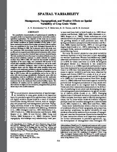
McBratney and Pringle, 1998; Mueller and Pierce, 2003; Terra et al., 2004). Hence, spatial methods of analysis have a potential for providing soil C researchers with a powerful analysis tool that could enable detection of smaller differences between management treatments. Smaller differences in soil C can be generated by management effects in a shorter experimental time, thus, at less expense. An additional benefit to soil C researchers is the ability to use secondary information from experimental sites in deciding on potential efficiency and usefulness of different data analysis methods. Topography is among the main factors driving spatial distribution and variability of soil C. Thus, for the experiments where soil C is the response variable topographical diversity of the experimental site might be an indicator of whether spatial methods should be considered. Thus, the objectives of this study are, first, to evaluate the potential performance of spatial methods of data analysis in small agricultural experiments where soil C is the primary variable of interest and to compare it with the performance of RCBD analysis and, second, to consider whether topographical characteristics of the potential experimental sites can be used by researchers as a decision guide for implementing spatial analyses. Based on comparisons between the methods of spatial analysis conducted by Zimmerman and Harville (1991), Brownie et al. (1993), and Wu and Dutilleul (1999), we use here only the methods that were found to be most effective in previous studies. Specifically, we consider, (i) analysis with spatially correlated residuals, and (ii) analysis with a trend and spatially correlated residuals. We use actual total soil C measurements rather than simulated data to ensure that variability from both spatial variability patterns and measurement errors reflects realistic field conditions. MATERIALS AND METHODS Data Collection and Preliminary Analyses Data for the study were obtained at the Kellogg Biological Station LTER site, in southwest Michigan (858249 W, 428249 N). For assessing performance of the spatial methods when soil C is the primary variable of interest we used total soil C data collected from 11 1-ha uniformly managed experimental LTER plots. For each plot the soil C data set consisted of approximately 35 to 45 geo-referenced random soil samples collected from 0- to 5-cm depth (Fig. 1). Samples were air-dried at room temperature, cleaned of visible plant residues and stones, and ground to pass a 2-mm sieve. Then, smaller visible plant material was removed by gentle air-blowing and samples were ground on a rolling grinder to pass a 100-mesh sieve. Total C was measured using a Carlo-Erba CN analyzer (Carlo Erba, Milan, Italy). To characterize variability of the total soil C in the studied plots we calculated statistical summaries and sample variograms, which were then fitted with variogram models. These tasks were accomplished using, respectively, PROC MEANS, PROC VARIOGRAM, and PROC MIXED procedures in SAS (SAS Institute, 2002). A total of 597 elevation measurements collected from the LTER site with land-based laser in 1988 (Robertson et al., 1997) were used to characterize topographical diversity of the studied plots. Distance between measurements ranged from 4

Fig. 1. Example of soil sample locations (solid circles) overlaid with a simulated experiment in one of the studied field sites.

to 20 m and approximately eight to nine elevation measurements were available for each plot. The elevation measurements were converted into a cell-based terrain map on a 15- by 15-m grid by means of inverse distance weighting with power of 2 and 6 nearest neighbors using ArcGIS 9.0 Spatial Analyst (ESRI, 2004). This terrain map has been reported by Kravchenko et al. (2005). Terrain slope and flow accumulation values were derived from elevation map using ArcGIS 9.0 Spatial Analyst (ESRI, 2004).

Experiment Simulations For experiment simulations we regarded each of the 11 experimental plots as a uniform separate field site with its corresponding set of soil C data. We will refer to the 11 LTER experimental plots as field sites and to the plots from the simulated experiments placed in these field sites simply as plots. To compare performance of the statistical analyses, the total soil C data sets from each field site were overlaid with simulated RCBD experiments (Fig. 1). A simulated experiment at each site consisted of three blocks with five plots per block for a total of 15 plots. The blocks were delineated based on closest proximity. Such block delineation is commonly used in setting up field experiments in sites with relatively flat terrain. The plots were 6 by 10 m in size and most of them contained three soil subsamples. Because of missing data several plots contained only one or two subsamples. Five fictitious treatments were assigned at random to the plots within each block. No treatment effect was simulated, that is, only the original soil C measurements were used in the data analyses. A total of 15 simulated experiments were conducted at each site. Each simulated experiment consisted of a different random assignment of treatments to the experimental plots, that is, a total of 15 randomizations were performed for each of the 11 field sites. The 15 simulated experiments were not related to the total number of plots. It was just a feasible number of randomizations that produced convincing results on method comparisons.

Description of Spatial Methods of Analysis Theoretical aspects of the spatial analysis used in this study, known as random field analysis, are developed by Zimmerman


KRAVCHENKO ET AL.: USING SPATIAL VARIABILITY TO ESTIMATE SOIL C

825

and Harville (1991), and are described in detail in a number of other studies (e.g., Zimmerman and Harville, 1991; Brownie et al., 1993; Stroup, 2002; Hong et al., 2005). Hence, we will provide only a brief overview of the statistical methods we used. First, we looked at a classical RCBD analysis, which remains the most commonly used type of analysis for RCB field experimental designs. Statistical model for soil C observations (yij) in a RCBD analysis consists of treatment and block effects and residuals,

The second spatial analysis considered in this study is the random field analysis with trend and spatially correlated residuals (SA2), which was found to be superior to other spatial analyses in a number of other studies (e.g., Zimmerman and Harville, 1991; Brownie et al., 1993). The underlying statistical model of this analysis consists of fixed effects of treatments and fixed effects of the functions of location of the experimental units, that is x and y coordinates of plots. For illustration, model with linear trend in x and y direction is,

yij 5 m 1 Blocki 1 trtj 1 eij

yij 5 m 1 trtj 1 xij 1 yij 1 eij

where i the block number, j is the treatment number, m is the overall mean, Blocki is the random effect of blocks, trtj is the fixed effect of the treatments and eij are the residuals. The residuals are assumed to be independent and normally distributed with zero mean and a constant variance, s2. Thus, the covariance matrix for the residuals, R, consists of zero offdiagonal covariance, s2, elements, which correspond to zero correlation between the plots separated by distance h,

The residuals are assumed to be correlated and their covariance structure is modeled as described above for SA1. We were concerned that in the small simulated experiments of this study the number of plots might be insufficient for adequate modeling of the spatial trend. Thus, we also considered a modified version of SA2 method (SA2a). In SA2a, instead of plot averages, we used geo-referenced location and soil C information of every individual subsample, hypothesizing that more numerous geo-referenced subsample data would allow for more accurate estimation of the trend parameters. The statistical model with linear trend in x and y direction based on subsample data is

R 5 s2 In where In is the identity matrix of rank equal to the number of the plots, n. In this analysis we assumed that unbalance due to somewhat unequal number of subsamples per plot is negligible and used averages of soil C data obtained based on the subsamples available in each plot. This is consistent with a typical field experiment where one composite soil sample is collected per plot based on several soil cores. We assumed that the average of the subsamples in our simulated experiments is equivalent to a composite plot sample. The first spatial analysis method that we considered is the random field analysis with correlated errors (SA1). The main difference of SA1 method from RCBD is its approach to residuals. Unlike in a traditional analysis of variance the residuals are not assumed to be independent from each other, but correlated. Their correlations reflect the spatial structure in variability of the studied property with expectation that observations/residuals closely located are more similar to each other than those separated by greater distance. Parameters describing the spatial structure form a basis for the covariance matrix of the residuals, R, in the SA1 statistical model. Thus, spatial structure is accounted for by modeling covariance structure of the residuals. The statistical model for the analysis consists of only treatment effects and residuals,

yij 5 m 1 trtj 1 eij where the residuals are correlated. The model does not include the block effects since it is assumed that the block effect is being accounted for by modeling correlation among the residuals. Spatial correlation as a function of separation distance h is commonly described and characterized using semivariograms, g(h), which are related to covariances, C(h), as C(h) 5 s2 2 g(h). Semivariogram models used in geostatistical applications, for example, spherical, exponential, Gaussian, are usually employed to model the covariance structure of the spatially correlated residuals. For illustration, if the spatial structure of the residuals is represented by an exponential model, then the covariance, s2ij, elements of the R matrix are obtained as

s2ij 5 C(h) 5 s2 exp(2h/a) where s2ij is the covariance between the two plots, i and j, separated by distance h, and a is the spatial correlation range. In theory, the R from spatially correlated residuals would lead to lower values of standard errors for treatments and contrasts between the treatments and, thus, to more efficient analysis.

yijk 5 m 1 trtj 1 eij 1 xijk 1 yijk 1 dijk where k is the subsample within each plot, eij are the residuals associated with variations between the plots and dijk are residuals associated with subsamples. The subsamples are assumed to be spatially correlated with each other and the covariance structure is modeled for the subsample residuals. In the SA2 (analysis based on the plot locations) the order of the polynomial function used in the model was limited to two for x coordinate and one for y coordinate. For the SA2a (analysis based on subsample locations) we used the polynomial functions of the x and y coordinates up to the fourth order. Only the trend components significant at P , 0.01 were kept in the analysis following recommendations of Tamura et al. (1988) and Brownie et al. (1993). The analyses were conducted using PROC MIXED procedure in SAS. For each analysis that involved modeling covariance structure of the residuals we considered three functions, namely, spherical, exponential, and Gaussian. For each function two parameters, that is, residual variance, s2, and spatial correlation range, a, were estimated by restricted maximum likelihood, a default method of PROC MIXED. Log-likelihood tests (Littell et al., 1996) showed that nugget effects were not significantly different from zero (P , 0.05) thus were not included in the models. After estimation of the spatial covariance model parameters, the restricted maximum likelihood procedure then uses them to obtain estimates of treatment effects along with variances/standard errors for the treatment effects and comparisons between the treatments.

Performance Comparison Criteria To compare performance of statistical models of the studied analyses we used the Akaike Information Criterion (AIC), as described in Littell et al. (1996). The AIC is calculated based on log-likelihood values taking into account the number of model parameters. Lower AIC values indicate better performing statistical model. For the outcome of each of the 15 randomizations in each field site, the AIC values of RCBD analysis were compared with those of SA1, SA2, and SA2a analyses. If RCBD analysis produced the lowest AIC value it was concluded that RCBD model was the optimal for the outcome of a given randomization in a given field site and spatial analyses were considered no further. When AIC values


826


of spatial analyses were less than those of RCBD we proceeded with comparing analysis efficiencies. As a criterion of efficiency of the analysis we used the average standard error obtained by averaging standard errors from all pair-wise comparisons between the treatment means (Zimmerman and Harville, 1991; Brownie et al., 1993; Qiao et al., 2000). The smaller the standard error for difference among treatment means the smaller are the differences between the treatments that can be detected by using a certain statistical analysis, thus, the higher the efficiency of that statistical analysis.

viously, the strength and extent of spatial correlation are important in defining how well the spatial analyses perform. Thus, we illustrated power calculations using three different spatial correlation ranges. The spatial correlation ranges considered were 15, 25, and 35 m. The minimum difference/ number of replication curves were developed based on the pooled value of the variance obtained from total C data from all 11 data sets, equal to 0.041. For RCBD analysis we used estimated error and block variances of 0.026 and 0.015, respectively, obtained also based on pooled estimates from the simulated experiments of the studied 11 field data sets.

Power Analysis Illustration

RESULTS AND DISCUSSION

Since there was no treatment effect in the simulated experiments of this study only comparisons in efficiency based on average standard errors were possible. Thus, we decided to further illustrate how higher efficiency of the analysis may translate into smaller statistically detectable differences in total soil C between the treatments. For that we conducted a power analysis using the approach outlined by Stroup (2002) using SA1 method as an example and we compared the results with those of RCBD analysis. We computed the numbers of replications (plots per treatment) needed to declare a certain difference between the treatments to be statistically significant at a 5 0.05 with power of 0.80. To obtain the differences we designated one of the fictitious treatments to be a treatment that increases total soil C values, while all the other treatments were assumed not to contribute to an increase in soil C. To model these treatment effects the difference between the treatments was added to the first treatment while the remaining treatments remained intact. We studied the differences that could be detected with number of replications ranging from 2 to 10. As mentioned pre-

A summary of the total C data for the studied field sites is shown in Table 1 along with variogram model parameters obtained by fitting sample variograms of the studied data sets. Total soil C ranged from 0.64% (field site 4) to 1.32% (field site 9) with coefficients of variation as low as 9.1% in field site 1 to as high as 27.7% in field site 10. Spatial variability characteristics of the studied data sets were also quite diverse ranging from no noticeable spatial correlation present (field sites 1 and 2) to strong spatial correlation. Strong spatial correlation with low nugget/sill ratios and relatively large spatial correlation ranges was observed in field sites 7, 8, 9, 10, and 11.

Overall Comparisons between the Methods of Data Analysis In comparing performance of the studied statistical procedures we found that SA2 method, that is, spatial

Table 1. Statistical and geostatistical summaries of the total soil C data from the 11 studied field sites along with selected topographical characteristics of the studied sites. Statistical summary Field site 1 2 3 4 5 6 7 8 9 10 11

Geostatistical summary

No. of soil samples

Mean

Range

CV†

Variogram model

Nugget

Sill

Nugget/sill ratio

Spatial correlation range

41 39 44 39 37 42 37 42 42 42 44

% 0.78 1.15 0.79 0.64 1.08 1.11 0.96 1.25 1.32 1.22 0.97

0.39 0.69 0.45 0.47 0.69 1.02 0.58 0.91 1.01 1.37 0.78

% 9.1 13.9 14.0 18.4 17.8 26.6 12.8 20.5 16.9 27.7 17.5

nugget nugget spherical spherical spherical spherical spherical Gaussian spherical spherical spherical

0.005 0.025 0.002 0.008 0.007 0.028 0.002 0.008 0.000 0.003 0.003

0.005 0.025 0.014 0.016 0.037 0.084 0.026 0.088 0.060 0.084 0.031

% 100 100 15 50 19 33 8 9 0 4 10

m NA NA 15 48 29 35 64 22 36 29 25

Topographical characteristics Field site 1 2 3 4 5 6 7 8 9 10 11 † CV, coefficient of variation.

Elevation range

Maximum slope

Maximum flow accumulation

m 0.4 0.4 0.5 0.8 0.5 0.5 0.4 0.9 0.2 0.3 0.4

degrees 0.7 0.7 0.7 1.6 0.9 1.1 0.9 1.5 1.1 1.1 0.8

25 47 36 25 21 64 106 216 197 154 6

827

analysis with trend and correlated residuals based on plot data, was an unacceptable choice of data analysis in these small-sized experiments. In 8 of 11 field sites none of the trend components were found to be statistically significant (P , 0.01). In the remaining three field sites, this analysis produced inconsistent results in terms of hypothesis testing. Thus the trend analysis with correlated errors was not further pursued. Poor performance of this analysis is an expected result of the small size of the studied data sets (only 15 plot data points). Performance of the SA1 and SA2a methods varied in different field sites. In 9 of the studied 11 data sets the AIC values from at least one of the two studied spatial analyses in either all or in the majority of the 15 randomizations were lower than those from RCBD. This indicates that the statistical models that accounted for spatial correlation were preferable to the RCBD model in these field sites. Spatial analyses were not considered further in the two field sites where RCBD produced the lowest AIC values in majority of 15 randomizations (Table 2). Average standard errors from all pair-wise comparisons between the treatment means were calculated based on both RCBD and SA1 and SA2a analyses for the nine field sites where spatial models produced lower AIC values than those of RCBD. In eight of these nine field sites the average standard errors from at least one of the two studied spatial analyses were lower than those of the RCBD analysis. Thus, the minimum differences between the treatments, which could be detected statistically with a certain level of significance, were lower if data from these field sites were analyzed via spatial methods instead of traditional RCBD analysis. Note, that although the simulated experiment had only 15 plots, even in these small data sets the spatial structure was successfully modeled with the spatial anTable 2. Average standard errors from all pairwise comparisons between treatment means for the three studied statistical analyses. The values in the table are averages from 15 randomizations. For each field site the values are shown only for the spatial analyses that converged and produced Akaike Information Criterion (AIC) values less than those of randomized complete block design (RCBD) in at least 8 out of 15 randomizations. In parenthesis are shown the percent of improvement in the standard error of the spatial analysis as compared with RCBD. Avg. standard errors Field site 1 2 3 4 5 6 7 8 9 10 11

RCBD

SA1†

SA2a‡

0.039 0.071 0.058 0.062 0.083 0.183 0.072 0.135 0.108 0.238 0.087

NA§ NA 0.063 (28.6) 0.055 (11.3) NA 0.136 (25.7) 0.064 (11.1) 0.095 (29.6) 0.081 (25.0) 0.133 (44.1) 0.073 (16.1)

NA NA NA NA 0.082 (1.2) NA 0.060 (16.7) 0.060 (55.6) 0.083 (23.1) 0.113 (52.5) 0.072 (17.2)

† SA1, random field analysis with correlated errors based on plot data. ‡ SA2a, random field analysis with trend and correlated errors based on subsample data. § NA, fewer than 8 of 15 randomizations converged and produced AIC values lower than that of RCBD analysis.

alysis based on plot data (SA1), making it preferable to and more efficient than RCBD in 7 of the studied 11 field sites. The results support our hypothesis that when strong spatial correlation is present in soil C distribution, the spatial analysis will perform with higher efficiency than RCBD even in small sized experiments. The SA2a method was more efficient than the SA1 method in five of the studied field sites (Table 2). However, only in field sites 8 and 10 was the improvement in efficiency substantial. The best performance for the SA2a method was observed in field site 8 where it produced a 55.6% improvement in standard error over RCBD as compared to 29.6% improvement of SA1 method.

Effects of Individual Site Characteristics on Method Performances The variations in performance of spatial methods in different field sites were associated with differences in topographical diversity and variability in the strength of spatial structure, which for soil C is itself to a large extent a function of topographical diversity. The two of the field sites (field sites 1 and 2), where none of the studied spatial methods of data analysis produced lower AIC values than RCBD analysis, were the field sites with somewhat lower variability of total C (Table 1). The field site 1 had the smallest range of C values among the 11 studied field sites. Coefficients of variation (CV) for these two field sites were among the lowest of the studied data (Table 1). Spatial variability characteristics indicated no spatial structure. The sample variograms for soil C data of the sites 1 and 2 were best modeled by pure nugget effect model. As an example, the sample variogram for data set 2 is shown in Fig. 2. The topography of these sites was also among the flattest, with terrain slopes of 0.7 degrees (Table 1). In field sites 3 to 6 at least one of the two studied spatial analyses had lower AIC value than RCBD in at least 8 of the 15 randomizations. Overall variability, that is, CV values of soil C in these field sites, was higher than that of the field sites 1 and 2. The spatial structure was evident in the sample variograms. However, in some 0.1

Field site 2 Variogram ( γ (h))



0.08

Field site 9 Field site 5

0.06 0.04 0.02 0 0

10

20

30

40

50

Distance (h), m Fig. 2. Example of sample variograms for total soil C from three of the studied field sites and the variogram models fitted to the sample variograms by restricted maximum likelihood method in PROC MIXED (SAS). Model parameters are shown in Table 1.


828


cases (field site 3) the spatial correlation range was relatively small (15 m) as compared to dimensions of the plots (6 by 10 m). In other field sites the nugget/sill ratio was relatively high, for example, 50 and 33% in field sites 4 and 6, respectively. As an example of a typical variogram for this group of field sites, the sample variogram for field site 5 is shown on Fig. 2. The topography of these sites was somewhat more diverse than that of the field sites 1 and 2. The terrain slopes were higher than 0.7 in these field sites, and the range of elevations was also often larger than that of the field sites 1 and 2. In five of the studied field sites (field sites 7–11) both spatial methods of data analysis produced lower AIC values than RCBD and lower average standard errors than those of RCBD in every one of the 15 randomizations (Table 2). Except for field site 7, these sites had the higher ranges of soil C values and higher CV values than those of field sites 1 and 2. They all had an overall stronger spatial correlation than the other field sites in the study. The nugget/sill ratios from the variograms of these data sets were lower than in all other data sets. Example of a sample variogram for these sites (field site 9) is shown on Fig. 2. Field sites 8 to 10 had aboveaverage terrain slopes. Field sites 7 to 10 also had the highest values of maximum flow accumulation among the studied 11 sites. High flow accumulation values usually correspond to the concave areas that accumulate water flowing from the surrounding terrain. Thus, the field sites that include such areas have more distinct patterns in spatial distribution of soil C reflected in stronger spatial correlation.

Minimum Detectable Differences Power curves reflecting relationships between the number of replications (blocks) and the minimum difference between the treatments that can be detected as statistically significant at certain level of significance are shown in Fig. 3. For the spatial correlation range of 15 m,

Fig. 3. Relationships between the number of replications and the difference in total soil C (%) between the treatments that can be detected as statistically significant via F-test for treatment effects with power of 0.80 and a of 0.05 using standard randomized complete block design (RCBD) analysis and random field analysis with correlated errors based on plot data (SA1) analysis with spatial correlation ranges of 15, 25, and 35 m.

comparable to the plot size (10 by 6 m), minimum detectable differences of SA1 are not different from those obtained in a standard RCBD analysis. For example, the minimum difference that can be detected by both RCBD and SA1 methods in an experiment with three replications, plot size of 6 by 10 m, and spatial correlation range of 15 m is equal to 0.45% (Fig. 3). However, at larger spatial correlation ranges (25 and 35 m) minimum detectable differences of SA1 are smaller and the spatial analysis thus more efficient as compared with the RCBD approach. For example, in an experiment with three replications and plot size of 6 by 10 m the minimum detectable differences in total C obtained by SA1 are equal to 0.30 and 0.25% for 25- and 35-m spatial correlation ranges, respectively. That is, it is substantially lower than the difference that is detected by RCBD analysis (Fig. 3). Thus, accounting for spatial correlation can lead to substantial reduction in number of samples in soil C related studies as compared to the numbers of samples reported previously (Garten and Ashwood, 2002). Consistent with conclusions of Stroup (2002), we also note the importance of a properly blocked and randomized experiment for efficient performance of spatial analyses. Power analysis conducted using an RCBD experimental set up with treatments assigned to experimental plots in a systematic and not a random manner resulted in much poorer performance of the spatial analysis as compared to that in a properly randomized experiment (data not shown).

CONCLUSIONS This study compared the performance of spatial methods of data analysis with RCBD analysis for simulated experiments based on total soil C data collected at 11 studied locations. The simulated experiments consisted of five treatments and had only three replications with approximately three subsamples collected from each plot. However, even in such relatively small experiments, statistical analyses that accounted for spatial variability were found to be more efficient than the RCBD analysis for a majority of the field sites. The results support our hypothesis that strong spatial correlation intrinsic to spatial distribution of soil C makes accounting for spatial variability beneficial for improving the efficiency of statistical analyses even in field experiments with moderate number of soil samples. As expected, performance of the spatial analyses depended on the strength of spatial variability in the studied sites. In sites where strong spatial structure was observed for soil C distribution, spatial analyses were preferable to RCBD. In most instances, spatial analyses produced consistently lower standard errors which would result in lower minimum detectable differences between treatments than those of RCBD analysis. We found that topographical diversity was a good indicator of the strength of spatial correlation in soil C and thus, of the potential efficiency of the spatial analyses. In the sites with more diverse terrain spatial analyses were more efficient than RCBD. Note that the topographic



diversity of the studied fields can be regarded as overall low with terrain slopes of the field sites not exceeding 2 degrees. However, even in this relatively flat topography spatial correlation in soil C distribution was sufficiently strong for spatial analyses to produce more efficient results. Only in the field sites with the flattest terrain was the spatial structure of soil C distribution negligible and thus there were no advantages to use spatial analysis. We believe that using spatial analyses will be even more advantageous when the experiments are placed in sites with more diverse terrain than that of this study. Power analysis supported the empirical observations from the studied sites indicating higher efficiency of the spatial analysis in data sets with large spatial correlation ranges as compared to standard RCBD analysis. ACKNOWLEDGMENTS This research was sponsored by USDA Sustainable Agriculture Grant and MSU Intramural Research Grant, it was also supported by the NSF Long-Term Ecological Research, Project No. DEB98-10220 at the Kellogg Biological Station and by the Michigan Agricultural Experiment Station. We thank Matias Ruffo and Ignacio Colonna (graduate students with Dr. Don Bullock from the Department of Crop Sciences, University of Illinois, Champaign-Urbana) for their help on collecting elevation data and the LTER team for help with collecting soil samples.

REFERENCES Ball, S.T., D.J. Mulla, and C.F. Konzak. 1993. Spatial heterogeneity affects variety trial interpretation. Crop Sci. 33:931–935. Besag, J., and R. Kempton. 1986. Statistical analysis of field experiments using neighbouring plots. Biometrics 42:231–251. Bhatti, A.U., D.J. Mulla, F.E. Koehler, and A.H. Gurmani. 1991. Identifying and removing spatial correlation from yield experiments. Soil Sci. Soc. Am. J. 55:1523–1528. Bowman, D.T. 1990. Trend analysis to improve efficiency of agronomic trials in flue-cured tobacco. Agron. J. 82:499–501. Brownie, C., D.T. Bowman, and J.W. Burton. 1993. Estimating spatial variation in analysis of data from yield trials, a comparison of methods. Agron. J. 85:1244–1253. Cambardella, C.A., T.B. Moorman, J.M. Novak, T.B. Parkin, D.L. Karlen, R.F. Turco, and A.E. Konopka. 1994. Field-scale variability of soil properties in Central Iowa soils. Soil Sci. Soc. Am. J. 58: 1501–1511. Cargnelutti, A., L. Storck, and A.D. Lucio. 2003. Adjustments of error mean square in corn cultivar competition trials by Papadakis method. Pesqui. Agropecu. Bras. 38:467–473. Casler, M.D. 1999. Spatial variation affects precision of perennial coolseason forage grass trials. Agron. J. 91:75–81. Duarte, J.B., and R. Vencovsky. 2005. Spatial statistical analysis and selection of genotypes in plant breeding. Pesqui. Agropecu. Bras. 40:107–114. Environmental Systems Research Institute. 2004. ArcGIS Spatial Analyst. ESRI, Redlands, CA. Garten, C.T., and T.L. Ashwood. 2002. Landscape level differences in soil carbon and nitrogen: Implications for soil carbon sequestration. Global Biogeochem. Cycles 16:1114. Hamann, A., G. Namkoong, and M.P. Koshy. 2002. Improving precision of breeding values by removing spatially autocorrelated variation in forestry field experiments. Silvae Genet. 51:210–215.

829

Hong, N., J.G. White, M.L. Grumpertz, and R. Weisz. 2005. Spatial analyses of precision agriculture treatments in randomized complete blocks: Guidelines for covariance model selection. Agron. J. 97:1082–1096. Kempton, R.A., and C.W. Howes. 1981. The use of neighbouring plot values in the analysis of variety trials. Appl. Stat. 30:59–70. Kirk, H.J., F.L. Haynes, and R.J. Monroe. 1980. Application of trend analysis to horticultural field trials. J. Am. Soc. Hortic. Sci. 105:189–193. Kravchenko, A.N. 2003. Effect of spatial structure on mapping accuracy and performance of interpolation methods. Soil Sci. Soc. Am. J. 67:1564–1571. Kravchenko, A.N., G.P. Robertson, K.D. Thelen, and R.R. Harwood. 2005. Management, topographical, and weather effects on spatial variability of crop grain yields. Agron. J. 97:514–523. Littell, R.C., G.A. Milliken, W.W. Stroup, and R.D. Wolfinger. 1996. SAS system for mixed models. SAS Inst., Cary, NC. McBratney, A.B., and M.J. Pringle. 1998. Estimating average and proportional variograms of soil properties and their potential use in precision agriculture. Precis. Agric. 1:125–152. Mueller, T.G., and F.J. Pierce. 2003. Soil carbon maps: Enhancing spatial estimates with simple terrain attributes at multiple scales. Soil Sci. Soc. Am. J. 67:258–267. Paul, E.A., K. Paustian, E.T. Elliott, and C.V. Cole (ed.) 1997. Soil organic matter in temperate ecosystems: Long-term experiments in North America. Lewis CRC Publ., Boca Raton, FL. Qiao, C.G., K.E. Basford, I.H. DeLacy, and M. Cooper. 2000. Evaluation of experimental designs and spatial analyses in wheat breeding trials. Theor. Appl. Genet. 100:9–16. Robertson, G.P., J.C. Crum, and B.G. Ellis. 1993. The spatial variability of soil resources following long-term disturbance. Oecologia 96: 451–456. Robertson, G.P., K.M. Klingensmith, M.J. Klug, E.A. Paul, J.C. Crum, and B.G. Ellis. 1997. Soil resources, microbial activity, and primary production across an agricultural ecosystem. Ecol. Appl. 7:158–170. SAS Institute. 2002. Statistics. Version 9.1. SAS Inst., Cary, NC. Schabenberger, O., and F.J. Pierce. 2002. Contemporary statistical models for the plant and soil sciences. CRC Press, Boca Raton, FL. Segovia-Lerma, A., L.W. Murray, M.S. Townsend, and I.M. Ray. 2004. Population-based diallel analyses among nine historically recognized alfalfa germplasms. Theor. Appl. Genet. 109:1568–1575. Smith, P. 2004. How long before a change in soil organic carbon can be detected? Glob. Change Biol. 10:1878–1883. Stroup, W.W. 2002. Power analysis based on spatial effects mixed models: A tool for comparing design and analysis strategies in the presence of spatial variability. J. Agric. Biol. Environ. Stat. 7: 491–511. Tamura, R.N., L.A. Nelson, and G.C. Naderman. 1988. An investigation of the validity and usefulness of trend analysis for field plot data. Agron. J. 80:712–718. Terra, J.A., J.N. Shaw, D.W. Reeves, R.L. Raper, E. van Santen, and P.L. Mask. 2004. Soil carbon relationships with terrain attributes, electrical conductivity, and a soil survey in a coastal plain landscape. Soil Sci. 169:819–831. Warren, J.A., and I. Mendez. 1982. Methods for estimating background variation in field experiements. Agron. J. 74:1004–1009. Weisz, R., B. Tarleton, J.P. Murphy, and F.L. Kolb. 2005. Identifying soft red winter wheat cultivars tolerant to Barley yellow dwarf virus. Plant Dis. 89:170–176. Wu, T., and P. Dutilleul. 1999. Validity and efficiency of neighbor analyses in comparison with classical complete and incomplete block analyses of field experiments. Agron. J. 91:721–731. Yang, R.C., T.Z. Ye, S.F. Blade, and M. Bandara. 2004. Efficiency of spatial analyses of field pea variety trials. Crop Sci. 44:49–55. Zimmerman, D.L., and D.A. Harville. 1991. A random field approach to the analyses of field-plot experiments and other spatial experiments. Biometrics 47:223–239.