Using infrared sensors for distance measurement ... - Semantic Scholar

OF

Robotics and Autonomous Systems 1006 (2002) 1–12

Using infrared sensors for distance measurement in mobile robots

4

G. Benet∗ , F. Blanes, J.E. Simó, P. Pérez

5 6

Departamento de Informática de Sistemas, Computadores y Automática, Universidad Politécnica de Valencia, P.O. Box 22012, 46080 Valencia, Spain

7

Received 9 August 2001; received in revised form 27 March 2002

DP RO

3

8 9

Abstract

18

Keywords: Infrared sensors; Distance measurement; Sensor models; Error estimation; Ultrasonic and infrared data integration

11 12 13 14 15 16

TE

17

The amplitude response of infrared (IR) sensors based on reflected amplitude of the surrounding objects is non-linear and depends on the reflectance characteristics of the object surface. As a result, the main use of IR sensors in robotics is for obstacle avoidance. Nevertheless, their inherently fast response is very attractive for enhancing the real-time operation of a mobile robot in, for instance, map building tasks. Thus, it seems that the development of new low-cost IR sensors able to accurately measure distances with reduced response times is worth researching. In this paper, a new IR sensor based on the light intensity back-scattered from objects and able to measure distances of up to 1 m is described. Also, the sensor model is described and the expected errors in distance estimates are analysed and modelled. Finally, the experimental results obtained are discussed. © 2002 Published by Elsevier Science B.V.

10

19

1. Introduction

21

Infrared (IR) sensors are widely used as proximity sensors and for obstacle avoidance in robotics. They offer lower cost and faster response times than ultrasonic (US) sensors. However, because of their non-linear behaviour and their dependence on the reflectance of surrounding objects, measurements based on the intensity of the back-scattered IR light are very imprecise for ranging purposes. For this reason, environment maps made with this type of sensor are of poor quality, and IR sensors are almost exclusively used as proximity detectors in mobile robots. However, some IR sensors described in the bibliography are based on the measurement of the phase shift, and offer medium resolution at long ranges (about 5 cm

24 25 26 27 28 29 30 31 32 33 34

RR

23

∗

CO

22

Corresponding author. Tel.: +34-96-387-75-78; fax: +34-96-387-75-79.

0921-8890/02/$ – see front matter © 2002 Published by Elsevier Science B.V. PII: S 0 9 2 1 - 8 8 9 0 ( 0 2 ) 0 0 2 7 1 - 3

UN

1 2

for distances up to 10 m [4]), but these are, in general, very expensive. US sensors are widely used for distance measurement purposes. They offer low cost and a precision of less than 1 cm in distance measurements of up to 6 m [1,4]. However, the most popular method used in these measurements is based on the time of flight (ToF) measurement. This ToF is the time elapsed between the emission and subsequent arrival after reflection of a US pulse train travelling at the speed of sound (approximately 340 m/s). This causes large response times (35 ms for objects placed 6 m away) for a single measurement. Moreover, the transducers used in robotics have wide angular sensitivity lobes (35◦ , typically), and offer poor angular resolution. IR sensors using reflected light intensity to estimate the distance from an object are not common, and only a small number have been reported in the bibliography [3,7–9]; but their inherently fast response is very attractive for enhancing the real-time response of a

EC

20

35 36 37 38 39 40 41 42 43 44 45 46 47 48 49 50 51 52 53 54

61 62 63 64 65 66 67 68 69 70 71 72 73 74 75 76 77 78 79 80 81 82 83 84 85 86 87 88 89 90 91 92 93 94 95 96 97 98 99 100 101 102

2. Description of the IR sensor

121

The IR sensor has been developed as a part of a mobile robot prototype called YAIR1 . This robot is a multi-sensor prototype being developed for research in several issues related with real-time distributed systems. YAIR has two main types of sensors for map-building and object location: an US rotary sensor placed on top, and a ring of 16 IR sensors distributed in eight pairs around the perimeter of the robot, as shown in Fig. 1. Each pair of sensors is centred at each edge of the octagon, with 15 cm of separation between them. The sensitivity lobes (corresponding to 50% of amplitude response) are also represented in this figure. The maximum detection range is approximately 1 m. The US sensor can measure distances with a precision of less than 1 cm, and with an angular positioning resolution of 1.8◦ . Response times vary from 15 ms for a single measurement to 2.5 s for a complete circular scan [2]. The IR sensors of the YAIR robot are based on the direct measurement of the magnitude of the IR light that is back-scattered from a surface placed in front of the sensor. Assuming perfect diffuse behaviour of

122

OF

60

DP RO

59

103

EC

58

uncertainties ranging from 0.1 mm for near objects to 10 cm for distant objects, being typically 1.2 cm objects placed at 50 cm. The organisation of this paper is as follows: Section 2 describes the IR sensor and its main characteristics, in Section 3 a simplified model with only one parameter (reflectivity coefficient αi ) is used to describe the sensor response as a function of distance and the angle of incidence. Section 4 describes the expected errors in obtaining distance measurements using the IR sensor—expressed as a function of the reading noise, distance, and angle of incidence. Section 5 describes a simple and accurate method to estimate the αi parameter, using US data readings as a complementary source of information. Also, in this section the influence of the αi parameter on the estimated distance is studied. Finally, in Section 6, the results obtained from several validation tests are described and discussed.

RR

57

mobile robot. Also, highly directional transducers are commercially available, giving better angular resolution than US transducers. Thus, it seems that the development of new low-cost IR sensors capable of accurately measuring distances with reduced response times is worth researching. Some low cost IR sensors based on the intensity of the reflected light have been reported. The sensor described [3,9] has poor range resolution and is only applicable for short distances (under 25 cm). In [10] a sensor offering an accuracy of 0.5 cm is described, but it only works over short distances (docking), and uses a priori known passive reflectors as position references. In [7], several IR-based distance sensors are analysed and compared, but none is fully satisfactory. In fact, the main application for IR sensors in mobile robots is collision avoidance rather than active range sensing. In an unknown environment, it is not possible to make valid assumptions about the nature of the surface properties of objects, and additional information sources are needed to obtain the relevant parameters of the surfaces. More specifically, to interpret sensor output as a distance measurement it is necessary to know how a given surface scatters, reflects, and absorbs IR energy [8]. Thus, to use IR in an unknown environment, the surface properties must be determined during robot operation. US sensors can be used as a complementary source of information to determine the surface properties. This co-operation between the US and IR sensors is not a new idea. In a classic paper [5], a navigation system that combines information from these two sensors to build a more accurate map is described. US and IR sensors are frequently used in a complementary way, where the advantages of one compensate for the disadvantages of the other. In [8], an IR sensor requiring a great deal of US co-operation to estimate the distance and angle of incidence from an object is described. In this paper, a new type of IR sensor is described. It is suitable for distance estimation and map building. Amplitude response as a function of distance and angle of incidence is easily formulated using a model that needs only one parameter: the IR reflection coefficient of the target surface. Once an object has been modelled and identified, its distance from the IR sensor can be obtained in successive readings, within 2 ms (typical response time). Distance measurements with this sensor can vary from a few centimetres to 1 m, with

CO

56

UN

55

G. Benet et al. / Robotics and Autonomous Systems 1006 (2002) 1–12

TE

2

1 YAIR stands for Yet Another Intelligent Robot, and is currently being developed under the grant CICYT TAP98-0333-C03-02 from the Spanish government.

104 105 106 107 108 109 110 111 112 113 114 115 116 117 118 119 120

123 124 125 126 127 128 129 130 131 132 133 134 135 136 137 138 139 140 141 142 143


3

148 149 150 151 152 153 154 155 156 157 158

159 160 161 162 163 164 165 166 167 168 169 170 171 172 173 174 175 176 177 178 179

3. Sensor model

180

The sensor output follows very closely the photometry inverse square law [6]. Thus, a simple equation can be used to model the sensor output s(x, θ) as a function of the distance x and the angle of incidence θ with the target surface: α s(x, θ) = 2 cos θ + β, (1) x

181

EC

147

where α and β are the model parameters. The α parameter includes: the radiant intensity of the IR emit-

RR

146

CO

145

the surface, the signal amplitude received is not linear with the distance, and follows an inverse square law [6] that depends on the distance to the object, angle of incidence, and the reflectance of the surface. Each sensor consists of two highly directional IR LED emitters and one PIN photodiode with a plastic daylight filter housing. The IR LEDs are connected in series with a resistor and driven by a NMOS transistor that is activated using a TTL compatible logic signal. The total IR LEDs current is 100 mA during the activation of the emission. Only one of the 16 pairs of LEDs is activated at each time. The equivalent diagram for one sensor can be seen in Fig. 2. The IR emitter has been chosen because it has a narrow half-angle (±10◦ ) and high radiant inten-

Fig. 2. Equivalent diagram of a single IR sensor. The IR activation and the output signals are multiplexed.

UN

144

TE

Fig. 1. Layout of the YAIR infrared ring. Shadowed sectors show the sensitivity lobes.

DP RO

OF

sity (80 mW/sr at 100 mA). The receiver photodiode is a fast device and has good spectral sensitivity (50 ␮A/(mW/cm2 ) at 900 nm), with a sensitive lobe of ±20◦ . The combination of the emitter–receiver can detect and measure distances to targets placed up to 1 m apart. If an object is placed in front of the sensor, the reflected light reaches the photodiode, and the corresponding photocurrent produces a voltage across a resistor placed in series with it. The voltage output of each one of the 16 sensors is multiplexed using a solid-state, low on-resistance, precision analogue multiplexer. This multiplexed voltage is amplified by a precision amplifier with adjustable gain and offset, giving an output voltage that ranges from 0 V (no object) to 5 V (white target placed at 10 cm). As the amplifier circuit uses ±12 V DC voltage supply, the output is linear within the whole output range, and no saturation is produced in the output signal. This amplified voltage is converted using a 10 bit semi-flash A/D converter with a total conversion time of 1 ␮s.

182 183 184 185

186 187


α = α0 αi .

194 195

198 199 200 201 202 203 204 205 206 207

208 209 210 211 212 213 214 215 216 217 218 219 220

221 222

223 224 225

226 227 228

(2)

The β parameter equals the amplifier’s offset plus ambient light effect. It can be obtained by taking a reading without IR emission. Under these conditions, this reading will correspond with the value of the parameter β. A new reading is taken immediately after IR emission is activated. By subtracting the previous reading, a signal without offset β is obtained. Thus, the influence of all the light sources, even fluorescent or incandescent lights, can be removed. By naming this ‘cleaned’ signal as y, Eq. (1) can be rewritten as α y(x, θ) = s(x, θ) − β = 2 cos θ. (3) x The influence of the angle of incidence is modelled in the above equations using the factor cos θ, assuming near-Lambertian perfect diffuse behaviour of the surfaces, following Lambert’s cosine law [6]. This assumption is invalid on some polished surfaces, but in our experience, most of the examined surfaces have shown satisfactory closeness to this law for angle values in the range [−45◦ , +45◦ ]. More complete models such as the Phong model [8] can be used instead, but they require more parameters to define the model and more complicated procedures to obtain these parameters.

To simplify subsequent expressions, the ratios R and R are defined as follows: x − x2 x1 − x2 R= , R = 1 (6) L L

248

and, from Fig. 3, the following expression can be written to obtain the apparent angle of incidence θ :

251

tan θ = R .

EC

193

229

(7)

This angle θ is close to, but is not, the true angle of incidence θ. As shown in Fig. 3, the true angle of incidence can be expressed as tan θ = R,

3.1. Model of the environment: Estimation of the angle of incidence θ

The distance between the IR sensor and an object can be estimated from the value of the reading y, using Eq. (3), as follows: √ α α x= cos θ. (4) cos θ = y y However, in real environments, the angle of incidence is a priori unknown. If an IR sensor detects the pres-

230 231 232 233 234 235 236 237 238 239 240 241 242 243 244 245 246

247

249

250

252 253 254 255 256

(8)

257

and from Eq. (4), the following relationships can be established: √ √ x1 = x1 cos θ, x2 = x2 cos θ, √ R = R cos θ. (9)

258

Now, using these relationships, Eq. (8) can be re-written as √ tan θ = R cos θ. (10)

263

RR

192

CO

191

UN

190

ence of a target in its sensitivity zone, the first approach is to suppose 0◦ as angle of incidence. Thus, the distance will be overestimated by a factor of cos θ. The greater the angle of incidence, the greater is the error obtained in the distance estimation. This makes it unadvisable to use this data to build an environment map, and a method to estimate the angle of incidence must be used. As shown in Fig. 1, the IR sensors are grouped into eight equally oriented pairs. Using the readings of one of these groups, a good estimate of the distance x and the angle of incidence θ can be obtained as follows. Fig. 3 shows a schematic of a group of two IR sensors, measuring a flat surface with an angle of incidence θ. Each sensor amplifies and measures the values of the signals y1 and y2 . As the angle of incidence is unknown, false estimates x1 and x2 for each distance are obtained assuming θ = 0◦ as a first approach: α α x1 = , x2 = . (5) y1 y2

OF

197

189

DP RO

196

ters, the spectral sensitivity of the photodiode, the gain of the amplifier, and the reflectivity coefficient of the target. The first three factors are constant, but the last factor is target dependent. Thus, the parameter α can be expressed as the product of two parameters, α0 and αi , being α0 constant for all the measurements and expressed in V m2 , and αi , a dimensionless reflectivity coefficient that can vary from 0 (black target) to 1 (white target). This parameter can be expressed as

188

TE

4

Therefore, to obtain θ, the following equations must be solved: 2

(R ) cos θ + cos θ − 1 = 0. 3

2

(11)

259 260 261 262

264 265 266 267 268

5

DP RO

OF


Fig. 3. Diagram for the angle of incidence estimation using two equally oriented IR sensors.

274 275 276 277 278

279 280 281 282 283 284 285 286 287 288 289 290 291 292 293 294 295

tan θ R = √ . cos θ

and the mean distance x can be calculated as follows: √ 1 1 x = x1 + x2 = x1 + x2 cos θ. (15) 2 2

305

4. Sources of error in distance estimates

307

Eq. (4) can be used to obtain an estimate of the distance x from the sensor reading (y), the angle of incidence (θ), and the reflectance coefficient of the target (αi ). Uncertainty in any of these values will produce uncertainty in the distance estimate. Assuming that αi is a parameter that can be estimated with sufficient precision (using other available sensory data, as explained later), the main sources of error are the noise in the measurement εy and the uncertainty in the angle of incidence, εθ . Thus, naming εxy as the error component caused by the noise in the reading εy , and εxθ as the error component due to the error in the angle of incidence estimation, the following equation can

308

(12)

Using the above equation (12), a set of values of R can be obtained from a set of values of θ, thus obtaining a set of pairs (R , θ) that can be used as a look-up table to compute θ by means a of simple linear interpolation. Alternatively, if an algebraic equation to obtain θ is preferred, it is a simple matter to adjust the above-mentioned set of pairs (R , θ) to an expression in the form:

3

θ = aR + bR .

TE

273

EC

272

RR

271

that only angles between −45◦ and 45◦ are of interest for this study, given that the octagonal layout of the IR ring of YAIR makes it difficult to obtain greater angles of incidence within the range of 1 m of distance.) After the estimation of the angle of incidence, it is now possible to obtain the compensated distances x1 and x2 , using the following formula: √ √ x1 = x1 cos θ, x2 = x2 cos θ, (14)

(13)

(R ,

In Fig. 4, a set of 100 pairs of values θ) has been plotted, corresponding with values of θ in the interval [−45◦ , 45◦ ]. This set of values has been adjusted using least-squares fit to determine a and b in Eq. (13), yielding the following results: a = 53.345441, b = −11.905434, with a standard error of 0.5830191◦ , and a correlation coefficient of 0.9997581. (Note

CO

270

This implies solving a cubic equation in cos θ, whose solution can be found in numerous maths books, but its exact solution implies a large amount of calculus. A faster approach can be used instead. Notice that in the above reasoning, the goal is to obtain the value of θ from the value of the ratio R calculated from the readings, and this implies solving a cubic equation (11). However, if the goal were to obtain R from θ, the solution would be trivial, re-writing the previous equation (10) as follows:

UN

269

296 297 298 299 300 301 302 303 304

306

309 310 311 312 313 314 315 316 317 318 319 320


DP RO

OF

6

325

326

327

328 329 330 331 332

333 334 335 336

and taking partial derivatives with respect to y and θ in Eq. (4), the following expressions can be obtained for the uncertainty of the estimate of the distance εx : x3 εxy = − εy , 2α cos θ x εxθ = − tan θεθ , 2

(17) (18)

x3 x εx = − (19) εy − tan θεθ . 2α cos θ 2 Assuming that εy and εθ are zero-mean, Gaussian, and uncorrelated noises with standard deviations σ y and σ θ , respectively, the standard deviation of the total uncertainty can be expressed as 2 2 x3 x σy + tan θ σθ . σx = (20) 2α cos θ 2 Some considerations on the magnitude of the errors produced in the distance estimation and their relationships are described below.

337

The value of the reading y includes a noise εy that is mainly due to the quantisation noise plus the amplification noise. It can be assumed that this noise is zero-mean and Gaussian. In the following discussion, normal incidence white targets are assumed (cos θ = 1 and αi = 1). Under these restrictions, and taking absolute values, Eq. (17) can be rewritten as

EC

324

(16)

εxy0 . =

RR

323

εx = εxy + εxθ

∂x ∂x = εy + εθ . ∂y ∂θ

CO

322

4.1. Uncertainty εy in the readings

be written:

UN

321

TE

Fig. 4. Plot of the values of the angle of incidence θ as a function of the ratio R .

x3 · εy . 2α

(21)

This shows that the uncertainty εxy0 in the distance estimation grows quickly with the cube of the distance x, and is inversely proportional to the parameter α. This relationship can also be used to evaluate the distance xmax that will produce a given maximum error in the distance estimate (εxymax ). Naming xmin as the distance that produces the full-scale reading (ymax ) when a white target (αi = 1, α = α0 ) is used, the following expression can be obtained from Eq. (4): α0 xmin = , (22) ymax

338 339 340 341 342 343 344 345

346 347 348 349 350 351 352 353 354 355

356


360 361 362 363

364

(23)

and substituting Eq. (23) for Eq. (21) and resolving xmax , it is finally possible to obtain for a white target and zero angle of incidence, the value of the maximum distance (xmax ) measurable with a given uncertainty (εxymax ): 2 3 2xmin εxymax xmax = . (24) εy /ymax

384

4.2. Uncertainty in the angle of incidence

369 370 371 372 373 374 375 376 377 378 379 380 381 382

385 386 387 388 389 390 391 392 393 394 395

396

From Eq. (4), it is evident that the angle of incidence plays an important role in distance estimation. The uncertainty εθ in the value of the angle of incidence θ produces an error εxθ in the distance estimate that has been expressed in Eq. (17). The above described method to obtain θ has been based on the readings y1 and y2 and therefore, is affected by the uncertainty on these values caused by noise εy . Thus, from Fig. 3, the following expression can be written to obtain the relationship between εθ and εy : (x1 + εx1y ) − (x2 + εx2y ) tan(θ + εθ ) = , L

(25)

x1 3 x2 3 εy1 − εy2 . 2αL 2αL

(26)

Moreover, taking into account the additive nature of noise and assuming that εy1 and εy2 are non-correlated, with the same variance σy 2 , the following expression can be obtained for the standard deviation of the angular noise: σθ = arctan tan θ +

σy x1 6 + x2 6 − θ. 2αL cos θ (27)

Note that in the above expression, x1 and x2 can also be expressed as a function of the mean distance x¯ = (x1 + x2 )/2 as follows: 1 x1 = x¯ + L tan θ, 2

1 x2 = x¯ − L tan θ. 2

(28)

397 398 399

400

401 402 403 404 405 406

407 408

409 410 411

412

4.3. Total error in the distance estimation

413

In Eq. (20) the expected standard deviation in distance estimation has been expressed as a function of the standard deviation of the reading error σ y , the angular error σ θ , the distance x, and the angle of incidence θ. Moreover, Eq. (27) shows the relationship between σ θ and σ y . Thus, for a given σ y , the expected error obtained in the distance estimation can be modelled using Eqs. (20) and (27), and will ultimately depend on the mean distance x¯ , and the angle of incidence θ. As an example, in Fig. 5, the values of the standard deviation of the error predicted by this model corresponding to a value of σy = 6 mV have been plotted (this is the value obtained in the real measurements for the prototype examined), for distances ranging between 10 cm and 1 m and for angles of incidence between −45◦ and +45◦ . As can be seen in Fig. 5, the minimum standard deviation of errors are produced with zero angle of incidence— being 6 cm at 1 m of distance, 1 cm at 55 cm, and 0.5 cm at 20 cm. This error increases with the angle of incidence and reaches 12.5 cm for ±45◦ at 1 m.

414

RR

368

CO

367

UN

366

tan(θ + εθ ) = tan θ +

EC

383

Under the assumption that the quantisation error is the main part of the noise εy , the term εy /ymax can be viewed as the effective resolution of the A/D converter. Thus, the full-scale range xmax of the sensor will be a compromise between the acceptable error in distance estimation, the minimum distance, and the effective bits of the A/D converter. As an example, by taking 10 cm as xmin , 5 cm as εxymax, and a 10 bit converter, Eq. (24) gives a maximum range of about 1 m. In addition, if the A/D resolution is 12 bit, then the maximum range obtained is 1.6 m. However, it is necessary to point out that it is not possible to reduce the noise without limitation, as the amplification noise has a non-zero value. In fact, it is difficult to reduce the noise in the measurement to below 5 mV. For this reason, if the full scale reading (ymax ) is 5 V, a 10 bit A/D converter seems to be a good choice.

365

and from the relationship between εxy and εy expressed in Eq. (21), the following expression can be obtained:

OF

359

α0 =

2 xmin ymax

DP RO

358

and the value of α0 can be obtained as

TE

357

7

415 416 417 418 419 420 421 422 423 424 425 426 427 428 429 430 431 432 433 434 435


DP RO

OF

8

Fig. 5. Standard deviation of the distance measurements predicted by the model described as a function of the mean distance to a surface and the angle of incidence.

441 442 443 444 445 446 447 448 449 450 451 452

453 454 455 456 457 458 459 460

TE

440

Throughout this paper, an exact knowledge of the value of αi is assumed, and a suitable method has been described to obtain its value using US data. However, it can be of interest to study the dependence of the uncertainty on the distance estimates as a function of the uncertainty in αi In practical situations, during a robot walk, single dark surfaces with unknown values of αi can be reached. Under these conditions, this object will be classified as too distant to collide. In a real scene, values of αi can greatly vary, meaning that typical relative errors in αi can reach up to ±40% if no method—such as that described in this paper—is used to measure them. This is the case of a surface with αi = 0.7, but with a value of αi = 1 or αi = 0.4 being used instead. Thus, a derivative-based method to obtain the error in distance estimates as a function of the uncertainty in αi will not be applicable in this case. In the following paragraphs, the error produced in the distance estimates is expressed as a function of the uncertainty in αi . Also, for this analysis, it is assumed that noise εy equals 0. Let us suppose that a surface with a reflectivity coefficient αi , is irradiated with a pair of robot IR sensors. Assuming, as a first approach, that the angle of incidence is 0, the same reading y will be obtained

EC

439

In the previous section, a priori knowledge of α0 and αi are assumed. As α0 is constant for each sensor and can be calculated using Eq. (23), the only parameter to be determined is αi (the relative IR reflectivity coefficient of the surface). To determine its value one must have additional sensory data. If US sensors are available, as is the case of YAIR, it is easy to obtain reasonably good values for αi . The method is simple: once a new object is localised, normal incidence is reached by means of rotation of the robot (the normal incidence is obtained when the readings of the two IR sensors are of the same value). Then, the US distance value (x) is estimated with sufficient precision. An estimate of αi can be obtained using the following equation:

5.1. Effects of uncertainty in αi

y¯ x2 αi = , α0

RR

438

5. Modelling the objects in the scene: Estimation of the αii parameter

(29)

where x is the value of the distance measured with the US sensor, and y¯ is the mean value of the readings taken from both IR sensors. Note that to obtain reasonable accuracy it is necessary to reduce the noise influence by taking sufficient readings from IR sensors. It is also preferable that the object is placed within a distance of 20 and 50 cm.

CO

437

UN

436

461

462 463 464 465 466 467 468 469 470 471 472 473 474 475 476 477 478 479 480 481 482 483 484 485 486 487


494

495 496 497 498

499 500 501 502 503 504 505 506 507 508 509 510 511 512 513

514 515 516

517 518 519 520 521 522

Thus, using the previous equations (30) and (31), the following equations can be obtained: αi x = x , (32) αi and by naming the uncertainty in αi as εα = αi − αi , the uncertainty in distance measurements εxα can be expressed as a function of uncertainty εα as follows: εxα εα x − x + 1 − 1. (33) = = x x αi As a rule of thumb, the previous equation indicates that the relative error obtained in the distance estimation is approximately half the relative error in the estimated αi . In effect, a relative error of 20% in αi produces approximately 10% of error in x (that is, 10 cm in 1 m). Note that the sign of errors in αi is the same as errors in x. The above Eq. (33) does not take into consideration the influence of the angle of incidence θ. This issue is to be faced in the following analysis. Assuming an angle of incidence θ with the irradiated surface, and using the previous Fig. 3, Eqs. (30)–(32) can be re-written. Thus, the readings obtained for each sensor will be the following: α0 α i α0 αi y1 = cos θ, y2 = cos θ, (34) x1 2 x2 2

OF

DP RO

493

TE

492

EC

491

and, if an erroneous αi is supposed, a false distance estimate x will be obtained instead: α0 αi . (31) x = y

3.1 assumes a previous knowledge of αi , but it still gives sufficiently good results for this case. Finally, using Eq. (15), an estimate for the mean distance x can be obtained. Given the nature of equations involved in this calculus, it is rather difficult to obtain an analytical expression for the error in distance estimation as a function of the distance using the described method. Instead, it is easier to plot a graphic representation of the error dependence with the angle of incidence. In Fig. 6, a family of curves showing the dependence of the absolute distance error values with the incidence angle θ and the relative error α /αi has been plotted. In Fig. 6, the mean distance x is 1 m, and the angle of incidence θ ranges between +40◦ and −40◦ . As expected, the error values corresponding with θ = 0◦ are the same as that obtained when using Eq. (33). Also, Fig. 6 shows that the angle of incidence has little effect on the error obtained in the distance estimation using the above described method, and the worst case is θ = 0◦ . As a conclusion for this study, the effect of uncertainty in the value of αi can be roughly modelled using Eq. (33), and ignoring the influence of the angle of incidence on this error. Also, from the same equation, the tolerable uncertainty in the estimated αi can be obtained for a given error in distance εxα . Note that this error is independent and uncorrelated with the read-

RR

490

(30)

and the non-compensated distance estimates (assuming an erroneous αi ) can be expressed as α α α0 αi 0 i x1 = , x2 = . (35) y1 y2

From these values, a false estimate θ will be obtained, and following the method described in Section 3.1 to determine the true angle θ, the compensated value of θ will be obtained using Eq. (13). This procedure is not entirely correct, as the method described in Section

CO

489

from each sensor: α0 αi y= 2 , x

UN

488

9

Fig. 6. Plot of the absolute error in distance estimates as a function of the angle of incidence θ and the relative error in αi . The mean distance x used in this plot is 1 m.

523 524 525 526 527 528 529 530 531 532 533 534 535 536 537 538 539 540 541 542 543 544 545 546 547 548 549


6. Experimental tests and model validation

558 559 560 561 562 563 564 565 566 567 568 569 570 571 572

Relative IR reflectivity (αi )

White cardboard Yellow cardboard Red cardboard Light blue cardboard Light green cardboard Cyan cardboard Light grey cardboard Brown cardboard Wooden panel Red brick wall Medium grey cardboard Concrete wall Black cardboard

1.00 0.99 0.98 0.97 0.94 0.91 0.90 0.78 0.77 0.61 0.59 0.53 0.12

In Fig. 7, the average of the 100 readings taken from each position, belonging to a single IR sensor, have been plotted. This figure shows that they follow very closely the theoretical curve modelled by Eq. (3) with α = 50 mV/m2 . In fact, the RMS error between these averaged points and the theoretical curve was only 2.3 mV, a value below the individual reading noise (6 mV). This indicates that the proposed equation (3) can be used to model the IR sensor output with sufficient precision.

EC

557

Material description

RR

556

The experiments were carried out using the frontal pair of IR sensors on a ring of the YAIR robot, whose layout has been previously described. The robot was programmed to follow a straight path in steps of 5.15 cm, ranging from 13.4 to 116.8 cm towards a Canson-type DIN A2-sized white cardboard. All the sensors were previously adjusted to give a full-scale reading (5 V) at 10 cm from the same white card with θ = 0◦ . Thus, the value of the parameter α0 for an adjusted sensor is 50.0 mV/m2 , assuming αi = 1 for the white card. From each of the 21 points, 100 readings were taken. Each measurement was taken in two phases: a first reading without IR emission (β parameter estimation), immediately followed by a reading with IR emission. The resolution of the A/D converter was 10 bit and the total time spent on the two consecutive readings was 2 ms. The precision in the x positioning of the robot was better than 0.5 mm.

CO

555

Fig. 7. Plot of the readings obtained from a single prototype IR sensor as a function of the distance of the white target. Each filled dot represents the average value of 100 readings taken from the same distance. The continuous line is the theoretical curve of the model expressed in Eq. (3), with α = 50 mV/m2 .

UN

552

OF

554

551

Table 1 Experimental values of αi for several surfaces

DP RO

553

ing noise εy . Thus, the total variance of the errors in distance measurement using the IR sensor will be obtained by adding the variances of the different sources of uncertainty described in this paper.

550

TE

10

573 574 575 576 577 578 579 580 581 582

11

DP RO

OF


587 588 589 590 591 592 593 594 595 596 597 598 599 600 601 602 603 604 605 606

EC

586

were obtained using a Canson paper that exhibits a near-Lambertian diffuse behaviour. On more polished surfaces, the results are poor with large angles, but good results can still be obtained by reducing the maximum angle of incidence.

607 608 609 610 611

7. Conclusions

612

In this paper, a new IR sensor based on the light intensity back-scattered from objects and able to measure distances of up to 1 m has been described. Also, a simplified expression is proposed for modelling the sensor response as a function of distance and angle of incidence. From this expression, the expected errors in distance estimates are analysed and modelled. The proposed model uses only one parameter: the reflection coefficient, αi . This approach gives satisfactory results for most surfaces. A simple method to estimate this αi parameter has also been presented, using US data as a complementary source of information. Also, the influence of uncertainty on the exact value of the relative reflectivity coefficient αi has been analysed, and an expression has been found to give a rough

613

RR

585

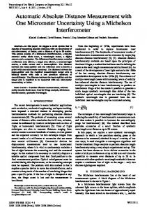
Also, different materials and surfaces were tested to prove the validity of the model, and similar results were obtained. In these tests, the value of the relative reflectivity (αi parameter) of each material has been previously obtained using Eq. (29). The values of αi for different materials are listed in Table 1. As can be seen, surface colour does not significantly alter the reflectivity values. In fact, almost all the coloured Canson-type cards show similar values for αi . To test the ability of the model to predict the angular response and the total estimation errors, similar experiments with the same white target were carried out, but for the following angles of incidence: 45, 30, 15, 0, −15, −30 and −45◦ . Using the above described procedure, the angle of incidence θ and the mean distance x from each pair of readings y1 and y2 were estimated using Eqs. (13) and (15), obtaining 100 estimates for each of the 21 different positions of the robot and for each of the indicated values of θ. With this set of estimates, the RMS error surface was obtained and plotted in Fig. 8. As can be seen, this RMS error surface shows values similar to those predicted in Fig. 5 by the proposed model. However, it must be pointed out that these satisfactory results

CO

584

UN

583

TE

Fig. 8. Plot of the total RMS error surface obtained in the distance estimation for each of the 21 × 7 different locations varying the distance and the angle of incidence, and taking 100 readings from each point.

614 615 616 617 618 619 620 621 622 623 624 625 626 627


641 642 643 644 645 646 647 648 649 650 651 652 653 654 655 656 657 658 659 660 661 662 663 664 665 666 667 668 669 670 671 672 673 674 675 676 677 678 679

[1] G. Benet, J. Albaladejo, A. Rodas, P.J. Gil, An intelligent ultrasonic sensor for ranging in an industrial distributed control system, in: Proceedings of the IFAC Symposium on Intelligent Components and Instruments for Control Applications, Malaga, Spain, May 1992, pp. 299–303. [2] F. Blanes, G. Benet, J.E. Simó, P. Pérez, Enhancing the real-time response of an ultrasonic sensor for map building tasks, in: Proceedings of the IEEE International Symposium on Industrial Electronics ISIE’99, Vol. III, Bled, Slovenia, July 1999, pp. 990–995. [3] V. Colla, A.M. Sabatini, A composite proximity sensor for target location and color estimation, in: Proceedings of the IMEKO Sixth International Symposium on Measurement and Control in Robotics, Brussels, 1996, pp. 134–139. [4] H.R. Everett, Sensors for Mobile Robots, AK Peters, Ltd., Wellesley, MA, 1995. [5] A.M. Flynn, Combining sonar and infrared sensors for mobile robot navigation, International Journal of Robotics Research 6 (7) (1988) 5–14. [6] Glassner, S. Andrew, Principles of Digital Image Synthesis, Vol. II, Kauffmann Publishers Inc., 1995. [7] L. Korba, S. Elgazzar, T. Welch, Active infrared sensors for mobile robots, IEEE-Transactions on Instrumentation and Measurement 2 (43) (1994) 283–287. [8] P.M. Novotny, N.J. Ferrier, Using infrared sensors and the Phong illumination model to measure distances, in: Proceedings of the International Conference on Robotics and Automation, Vol. 2, Detroit, MI, USA, April 1999, pp. 1644–1649. [9] A.M. Sabatini, V. Genovese, E. Guglielmelli, A low-cost, composite sensor array combining ultrasonic and infrared proximity sensors, in: Proceedings of the International Conference on Intelligent Robots and Systems (IROS), Vol. 3, Pittsburgh, PA, IEEE/RSJ, 1995, pp. 120–126. [10] P.M. Vaz, R. Ferreira, V. Grossmann, M.I. Ribeiro, Docking of a mobile platform based on infrared sensors, in: Proceedings of the 1997 IEEE International Symposium on Industrial Electronics, Vol. 2, Guimaraes, Portugal, July 1997, pp. 735–740.

634 635 636 637 638

F. Blanes received the M.S. degree (1994) and Ph.D. degree (2000) in computer engineering from the Universidad Politécnica de Valencia, Spain. Since 1995, he has taught real-time computer systems and he is currently an Assistant Professor in the Escuela Superior de Ingenier´ıa Industrial at the Universidad Politécnica de Valencia. His research interests include: real-time robot control, perception and sensor fu-

sion in mobile robots.

J.E. Simó received the M.S. degree in industrial engineering in 1990 from the Universidad Politécnica de Valencia (Spain) and a Ph.D. degree in computer science from the same university in 1997. Since 1990 he has been involved in several national and european research projects mainly related to real-time systems and artificial intelligence. He is currently an Associate Professor of computer engineering at the Technical University of Valencia and his current research is focused on the development of autonomous systems and mobile robots.

RR

633

CO

632

UN

631

OF

References

630

G. Benet received the M.S. and the Ph.D. degrees in industrial engineering from the Universidad Politécnica de Valencia, Spain, in 1980 and 1988, respectively. Since 1984 he has taught computed technology and currently he is an Associate Professor of the Escuela Universitaria de Informática at the Universidad Politécnica de Valencia. He has been involved in several national and european research projects mainly related to real-time systems and intelligent instrumentation. His research interests include: mobile robots, intelligent sensors, robot control and sensor data fusion.

DP RO

640

629

EC

639

estimate of the error produced in the distance estimation. Finally, the experimental results obtained show good agreement between the model and the real data obtained in the validation tests. Thus, this new sensor can be used in mobile robots to build reasonably accurate maps within real time constraints, given the fast response time of the IR sensor. Also, as an additional advantage of this sensor, each distance measurement can be obtained together with its expected uncertainty, enabling more accurate maps to be produced using simple sensor fusion techniques.

628

TE

12

networks.

P. Pérez received the M.S. (1998) degree from the Universidad Politécnica de Valencia, Spain. Since 1998, he has taught computer technology at Facultad de Informática. He is currently an Assistant Professor in the Departamento de Informática de Sistemas y Computadores at the Universidad Politécnica de Valencia. His research interests include: real-time robot control, embedded systems and field-bus