Using Instruction Sequence Abstraction for Shellcode Detection and ...

Using Instruction Sequence Abstraction for Shellcode Detection and Attribution Ziming Zhao and Gail-Joon Ahn Laboratory of Security Engineering for Future Computing (SEFCOM) Arizona State University, Tempe, AZ 85281, USA {zzhao30, gahn}@asu.edu Abstract—Although several research teams have focused on binary code injection, it is still an unsolved problem. Misuse-based detection lacks the flexibility to tackle unseen malicious code samples and anomaly-based detection on byte patterns is highly vulnerable to byte cramming and blending attacks. In addition, it is desperately needed to correlate newly-detected code injection instances with known samples for better understanding the attack events and tactically mitigating future threats. In this paper, we propose a technique for modeling shellcode detection and attribution through a novel feature extraction method, called instruction sequence abstraction, that extracts coarse-grained features from an instruction sequence. Our technique facilitates a Markovchain-based model for shellcode detection and support vector machines for encoded shellcode attribution. We also describe our experimental results on shellcode samples to demonstrate the effectiveness of our approach.

I.

I NTRODUCTION

Malicious binary code injection is still an unsolved problem that threatens critical net-centric production systems. Even though research efforts have been invested on such a devastating issue, production systems, where known vulnerabilities are not mitigated and potential vulnerabilities are introduced with newly-deployed modules, remain highly vulnerable to these threats. The injected malicious binary code is also known as shellcode since they used to return a command shell to the attackers. Misuse of informational data as executable code is the root cause of code injection attacks. Sanitization techniques that remove and escape reserved characters in the corresponding programming language are proven to be effective and efficient in scripting languages. However, these techniques are less successful in defending against binary code injection attacks due to the fact that there is no special meaningful token in binary to differentiate code from data. For instance, in IA-32 instruction set, the only invalid byte to start an instruction is 0xF1 and all other 255 possible values could be interpreted as the starting byte of a valid encoding [7]. Although signature-based methods remain the most effective ways to defeat known malware, they could be effective only when malicious samples have been acquired and signatures have been obtained. It is less useful against new samples and may be vulnerable to code encoding techniques, such as polymorphism and metamorphism. Several static analysis solutions [27], [8], [7], [30] construct some distinguishable criteria, such as the length of the instruction sequence, to identify previously unknown malicious code. Since the heuristics

in these methods are dependent on the existing knowledge of shellcode, they fail to accommodate the new trends of shellcode evolution. There also exist some discussions about utilizing both sequential and distributional byte patterns to model malicious code [28], [15]. However, statistically modeling the byte patterns is vulnerable to deliberate byte cramming [12] and blending attacks [13]. Moreover, quantitative analysis of the byte strength of different shellcode engines presented in [26] concludes that modeling the byte patterns in shellcode is infeasible. Besides all the investments on binary code detection, it is important to discover binary code attribution that automatically attributes binary code to its originating tools. Encoded shellcode attribution that tells whether the newly-captured shellcode sample is generated by a known shellcode engine provides security analysts and practitioners with more intelligence about the attack event and the adversaries behind the scene than simplistic detection approaches. However, existing work on this topic [16] that utilize byte characteristics still face the same challenges as binary code detection with byte anomaly analysis does. Consequently, systematic techniques that can confront the root cause of code injection, detect unseen malicious attacks and attribute newly-detected malicious code samples are imperative to cope with emerging rogue code threats and gather tactical intelligence for a more comprehensive knowledge base on cyberattacks. These solutions should be resilient to known attacks, such as byte cramming and blending, that undermine existing techniques. To achieve these goals, in this paper, we propose a novel solution based on static analysis and supervised machine learning techniques. Instead of using byte patterns, we propose instruction sequence abstraction to extract coarse-grained but distinguishable features from disassembled instruction sequence. We design a Markov-chain-based model and apply support vector machines for unknown shellcode detection and classification. The contributions of this paper are summarized as follows: •

We propose instruction sequence abstraction, a coarse-grained feature extraction method on the instruction sequence that reduces the size of input data dimension, removes confusing byte characteristics, and keeps distinguishable instruction features.

•

We design a Markov-chain-based model for shell-

code detection. Our detection approach is locationindependent and length-independent, hence it supports on-line shellcode detection on suspicious data streams. •

We apply support vector machines to capture distributional patterns shown in the instruction sequence abstraction for understanding encoded shellcode attribution.

•

The experimental evaluation with our proof-ofconcept system shows that our solution could (i) detect all types of unencoded shellcode from our dataset and (ii) attribute encoded shellcode to its originating engines with high accuracy.

The rest of this paper is organized as follows. Section II discusses the background and motivation of our solution. In Section III, we present our approach by illustrating the instruction sequence abstraction and proposing two learning models for shellcode detection and attribution. We show our experimental results in Section IV and discuss some research issues in Section V. Section VI overviews the related work and Section VII concludes the paper. II.

BACKGROUND AND M OTIVATION

In this section, we address the theoretical limit in differentiating code from data in IA-32 architecture. Then, we discuss why byte pattern analysis on this architecture is difficult. Also, we address some motivating examples observed in instruction sequences and discuss the challenges in using these characteristics. A. Differentiating Code from Data Accurate and robust methodology for differentiating code from data in a static way has a profound value for both programming language and computer security research. Disassembler and decompiler could use such technique to determine the boundary between code and data in file and memory for better understanding of programs without source code. Intrusion detection system could also make use of it to alert unseen cyberattack. For some computer architectures, this problem is trivial due to their instruction representations and memory alignments. However, some CISC architectures, such as IA-32, adopt variable-length instruction sets and permit interleaving of code and data. That is, instructions and data are stored together in the memory and have indistinguishable representations. The problem is even harder to solve when we consider self-modifying code and indirect jump (jmp eax)– a control transfer approach whose destination can only be calculated at execution time–in binary. Therefore, statically separating code from data in such architectures may lead to the halting problem that is undecidable in general [10], [31], [14], [18]. A major reason for the failure of byte pattern analysis on binary code is that even a slight change on assembly syntax would cause tremendous changes in byte syntax. Consequently, pattern detection and recognition on byte level is not resilient to assembly-level syntax change that is prevalent in shellcode encoding. For example, different shellcode instances from the same metamorphic engine could use different general registers to perform semantically equivalent

operations. While one could use two instructions pop edx; mov ebx, [edx] (byte sequence: 5A8B1A) to move a value from memory to register for computing, another may use pop eax; mov esi, [eax] (byte sequence: 588B30). Even though the instruction sequences look similar, the byte sequences only share one single byte (8B). With more sophisticated encoding technique, this shared byte could be further avoided. B. Motivating Examples Different from previous solutions that concentrate on byte patterns, we pay more attention on the instruction patterns shown in disassembly. We address instruction patterns of both sequences and distributions. Note that these patterns only serve as the motivation of our approach that is not dependent on any specific pattern mentioned in this section, but has the ability to extract human-observable and unobservable patterns in binary disassembly. A push-call sequential pattern consists of several push instructions followed by a call instruction. In IA32 architecture, the parameters to a function call are stored temporarily on stack usually by a push operation. Therefore, in a valid sequence of instructions, the subsequent instruction of push is more likely to be another push or call. A alphabet pattern is mostly found in shellcode generated by English shellcode [22] and alpha mixed encoder engines, whose outputs only consist of displayable ASCII values, such as English letters, blank space and punctuation marks. Because of the narrow choices these engines have, generated shellcode have significantly more unconditional jumps, stack and arithmetic operations than samples generated by other encoders. However, there are several obstacles in using these instruction observations directly in statistical models. For example, the trained model may overfit instruction patterns shown in the training set. Adversaries and encoding engines could easily choose other semantically-equivalent instructions to replace existing ones which render the modeling of any specific instruction ineffective. In order to solve these challenges, we propose instruction sequence abstraction, a coarse-grained feature extraction method, to tackle the problem of overfitting by mapping high-dimensional byte sequence representations to low-dimensional instances. III. Input Processor Training

Classifying

Shellcode

Suspicious Data Stream

O UR A PPROACH Feature Extractor Data Representations

Opcode Feature Extraction

Fig. 1.

Operand Feature Extraction

Customized Linear Sweep Disassembly

Instruction Sequence

1

2

Instruction Feature Extraction

Trainer and Classifier Training

Classifying

Learning Algorithms

Detection Algorithms

Markovbased Model

Detection Result Attribution Result

SVM Model

3

Our Approach Overview

A. Overview Our approach is based on static analysis and supervised machine learning as shown in Figure 1. Our solution consists

of three major components: i) input processor preprocesses binary code or suspicious data with customized linear disassembly that outputs the instruction sequence; ii) feature extractor reveals distinguishable features from the instruction sequence and outputs its two corresponding data representations named opcode mnemonic sequence and binary finite-dimensional representation; and iii) trainer utilizes Markov-chain-based model and support vector machines to train detection and classification models based on training set and classifiers that use trained models to detect and classify suspicious data. B. Customized Linear Sweep Disassembly The first step of our approach is to disassemble binary, a method that extracts semantics out of binary code and outputs machine-understandable disassembly. There exist two basic disassembly algorithms: i) linear sweep disassembly and ii) recursive descent disassembly. Linear sweep disassembly decodes new instruction at the location where the previous one ends. If the current byte could not be decoded as a valid starting byte of the instruction, linear sweep disassembly stops. The disadvantage of linear sweep disassembly is that it may mistakenly disassemble data as code if the starting location is wrong. Recursive descent disassembly determines whether a location should be decoded with the references by other instructions. In other words, recursive descent disassembly follows the control flow of the instruction sequence. Recursive descent disassembly stops when it could not determine the location of the next instruction, such as when an indirect jump is encountered. The major disadvantage of recursive descent disassembly is that it cannot cover the entire code section. In our solution, we need the most comprehensive coverage of disassembly. Therefore, we modify linear sweep disassembly and propose a customized linear sweep disassembly CLSD : (b1 , ..., bn ) → (i1 , ..., im ). Unlike linear sweep disassembly, CLSD does not stop when it reaches an undecodable address. Instead, it moves to the next address and perform linear sweep until it reaches the end of file. The complexity of this algorithm is O(n). Although CLSD may mistakenly decode some data section, such as encrypted payload in polymorphic shellcode, and incorrectly disassemble some instructions with a wrong starting location, this algorithm would disassemble the major portion of code over the data stream with the help of the selfrepairing ability of IA-32 instruction set [21]. C. Features In this section, we present our coarse-grained feature extraction method to reveal representative features from the instruction sequence (i1 , ..., im ) generated from CLSD. We try to introduce as many features as possible to reduce the possibility that the learned model is over-fitting the training dataset. We inspect both opcode and operand of an instruction as the sources for features. The opcode part of an instruction reveals the functionality of the disassembly statement, while operand part tells which object the effect is enforced on. We design opcode features based on two aspects: functionality and origin. Functionality captures the basic behavior and effect of a given opcode, and origin describes the source of instruction set that a given opcode was first introduced. Although the operand part of an instruction includes several fields such as addressing

form and immediate, for simplicity, we only analyze the usage of eight general purpose registers in an instruction as representative characteristics for operand features. We also use the length of instruction as a feature that represents the instruction in general. Opcode functionality: We categorize each opcode into one of the following ten groups in terms of its functionality: 1) Arithmetic. Opcodes that provide arithmetic operations, such as addition, multiplication, and some miscellaneous conversion instructions; 2) Shift, rotate and logical. Opcodes that provide shift, rotate and logical operations, such as bitwise and left shift with the carry-over ; 3) Unconditional data transfer. Operations that move data among memory locations and registers without querying flag register. Examples include mov, in, and out; 4) Conditional data transfer. Operations that move data among memory locations and registers based on the status indicated in a flag register. Examples include seta and setnl; 5) Processor control. Opcodes that manipulate the status of processor by modifying flag, loading and saving system registers, and synchronizing external devices. Examples include arpl, hlt, and lgdt; 6) Stack operation. Opcodes that manipulate a program stack. Examples include push, pop, enter, and leave; 7) Unconditional program transfer. Opcodes that change the program counter register without querying flag register. Examples include call, int, jmp, and ret; 8) Conditional program transfer. Opcodes that make transfer decisions based on specific bit combinations in flag register. Examples include ja, jne, and loopw; 9) Test and compare. Opcodes that compare the values of operands and store the result in some predefined register. Examples include test, cmp, and scas; and 10) Other operation. Opcodes that are not included in the aforementioned categories. Opcode origin: We also categorize each opcode into one of the following six instruction sets: 1) 8086 set, a group of instructions that were introduced with 8086 family CPUs [2]; 2) 80286, 80386, and 80486 sets. We combine these three instruction sets together because there do not exist many instances in each of these instruction sets; 3) Pentium and Pentium II sets; 4) 80387 and MMX, instruction sets that control and manipulate floating point coprocessors and MMX processors; 5) Pentium III and Pentium IV; and 6) Other sets. General register usage: For each instruction i in the instruction sequence, we analyze whether any of the eight general registers or any part of them is explicitly used in this instruction. These eight general registers are: 1) eax; 2) ebx; 3) ecx; 4) edx; 5) esi; 6) edi; 7) ebp; and 8) esp. For instance, in an instruction pop eax, the only explicitly mentioned general register is eax. We do not count the usage of esp because it is not explicitly mentioned in the operand part. For an instruction mov esi, [eax], both esi and eax appear in this statement. For an instruction add al, ch, we count one occurrence for both eax and ecx in this statement for the reason that al is part of eax and ch is part of ecx. Length of instruction: For each instruction i in the instruction sequence, we calculate its length. This feature is necessary because even instructions with the same opcode may vary in length. We split instructions into eight categories: Instructions

55 8BEC 8B7608 85F6 743B 8B7E0C 09FF 7434 31D2 (a) Byte sequence

are categorized into the first seven categories by using the length as an identifier if their lengths are not greater than seven bytes and instructions with longer than seven bytes fall into the eighth category. For example, mov ebp, esp (8BEC) is 2-byte long and classified in category ‘two’, and mov dword ptr [eax+ebp+14h], 0CCCCCCCCh (C7442814CCCCCCCC) is 8-byte long and falls into category ‘eight’.

push ebp mov ebp, esp mov esi, dword ptr [ebp+08] test esi, esi je 401045 mov edi, dword ptr [ebp+0c] or edi, edi je 401045 xor edx, edx (b) Instruction sequence

oT = (push, mov, mov, test, je, mov, or, je, xor) (c) OMS

D. Instruction Sequence Abstraction We now present instruction sequence abstraction which includes two representation methods to model instruction sequence: opcode mnemonic sequence (OMS) and binary finitedimensional representation (BFR). Since both methods map n-byte data sequence into much lower dimensional space as coarse-grained feature extraction approaches, they are abstractions of the original byte and the instruction sequence. While OMS maps instances in 256n byte sequence space to their counterparts in am space (a is the number of mnemonics in IA-32 instruction set and m is the length of the instruction sequence), BFR represents instances in Z32 space. For the mathematical notations, we use lower case bold roman letters such as f to denote vectors, subscript such as fi to denote the i-th component of f , superscript such as f (i) to denote the (i) i-th sample in dataset, and fj to denote the i-th sample’s j-th component. We assume all vectors to be column vectors and a superscript T to denote the transposition of a matrix or vector. Definition 1: Opcode Mnemonic Sequence (OMS). For a given instruction sequence i = (i1 , ..., im ), its opcode mnemonic sequence is represented as oT = (o1 , ..., om ), where ok ∈ {aaa, aad, ...}, which is the valid opcode mnemonic set of IA-32 architecture. Definition 2: Binary Finite-dimensional Representation (BFR). For a given instruction sequence i = (i1 , ..., im ), its binary finite-dimensional representation is a 32-dimensional vector f T = (f1 , ..., f32 ), where fi , i ∈ {1, ..., 10}, is the number of instructions in the i-th opcode functionality category, fi , i ∈ {11, ..., 16}, is the number of instructions from the corresponding opcode origins, fi , i ∈ {17, ..., 24}, is the occurrence of corresponding general register, and fi , i ∈ {25, ..., 32}, is the number of instructions with the corresponding length. Figure 2(b) shows the CLSD output of the byte sequence shown in Figure 2(a), and Figures 2(c) and 2(d) show the OMS and BFR representations of the example. E. Detecting Shellcode Based on the observation that certain instruction sequences are more likely to exist in some binary code rather than others, we propose to use the existence possibility of opcode mnemonic sequence to identify whether the suspicious byte stream contains shellcode. We choose first-order Markov chain, which is a discrete random process, to model the opcode mnemonic sequence by assigning each opcode mnemonic as a Markov state and computing the transition matrix of this Markov chain. Like other supervised machine learning techniques, our method has training and evaluation phases. Given OMSs of l shellcode training samples {o(i) }, i = {1, ..., l}, a transition

f T = (0, 2, 3, 0, 0, 1, 0, 2, 1, 0, 9, 0, 0, 0, 0, 0, 0, 0, 0, 2, 3, 3, 4, 1, 1, 5, 2, 0, 0, 0, 0, 0) (d) BFR

Fig. 2.

Instruction Sequence Abstraction Example

matrix P ∈ Ra×a can be trained, with the (i, j)-th element of P implies pij = P r(ok+1 = j|ok = i) indicating the probability of opcode state transition from ok to ok+1 . In the evaluation phase, we calculate shellcode probability score (Sscore) of suspicious data stream, which is defined in Definition 3 and determine whether it contains shellcode based on a threshold value t, which is also learned from the training set. Definition 3: Shellcode Probability Score (S-score). Given the transition matrix P trained from shellcode dataset and a suspicious OMS oT = (o1 , ..., om ), the S-score of this OMS is defined as follows: v u u k S-score(o) = t

max

i=1,...,m−k

i+k ∏

P r(oj+1 |oj )

(1)

j=i

where k is the length of calculation window. To calculate the S-score of o, a value for each of m−k opcode mnemonic subsequences with k-length is computed as the multiplications of the transition probabilities. Then, the maximum value among all m − k opcode mnemonic subsequences is chosen whose k-th root is defined as the S-score of o. If S-score(o) > t, we say the byte sequence where o is generated from is a shellcode and vice versa. Our shellcode detection approach is length-independent and location-independent on the byte sequence for two reasons: i) CLSD outputs the most comprehensive coverage of code, hence it has the ability to disassemble most shellcode bytes in a package, no matter where it is started; and ii) only the subsequent k instructions are used to calculate the S-score, hence the length of the byte sequence is not vital. Therefore, our approach is able to monitor on-line data stream, where the length and location of interesting points are unknown. F. Attributing Encoded Shellcode We propose to use support vector machines (SVM) to attribute encoded shellcode’s BFR to its originating encoding engine. SVM maps feature vectors into a higher dimensional space and computes a hyperplane to separate instances from different groups by maximizing the margin between them. Therefore, SVM is the largest margin classifier. The problem of attributing shellcode to its originating engine is a multiclass classification problem. However, the basic SVM only supports binary classification problems. Therefore, we use

algorithms that supports a one-vs-all approach to extend SVM for classifying multi-class problems. Here, we only discuss how to use SVM for the binary classification problem that checks whether a shellcode sample is from a specific engine e. Given l shellcode training samples {f (i) , y (i) }, i = 1, ..., l, where each sample is denoted by its BFR that has 32 features, represented as f (i) , and a class label yi with one of two values {-1|1}. -1 means it is not generated by an engine e, while 1 confirms a specific engine. The SVM requires the solution of the following optimization problem [4], [11], [6]: ∑ 1 T w w+C ξi 2 i=1 l

min

w,b,ξ

Subject to yi (w ϕ(f (i) ) + b) ≥ 1 − ξi , (2) ξi ≥ 0 where feature vectors f (i) are mapped to higher dimensional space by a function ϕ and C is the penalty parameter of the error term. In SVM, K(f (i) , f (j) ) = ϕ(f (i) )T ϕ(f (i) ), called the kernel function, determines how the feature vector maps data to higher dimensional space. It can be noted that the kernel function maps feature vectors into higher dimensional space only to search for a separate hyperplane so it does not rebuild more complicated features. Hence, it does not conflict with our approach to abstract features from the instruction sequence. T

IV.

E XPERIMENTAL E VALUATION

We first discuss the data collection and implementation details of our proof-of-concept system. Then, we present the shellcode detection and attribution results followed by the analysis approach for measuring the strength of 14 popular shellcode encoding engines. We conclude our evaluation with the performance of our system. A. Data Collection and Implementation We utilized Metasploit [23]–a penetration framework that hosts exploits and tools from a variety of sources–to collect shellcode samples. We collected 140 unencoded shellcode samples, all of which are executable on IA-32 architecture, across different operating system platforms including Windows (85), Unix (11), Linux (21), FreeBSD (10), OSX (12), and Solaris (1). These samples are used to train our Markovchain-based model and test the effectiveness of our approach. For the evaluation of encoded shellcode attribution, we chose 21 different payloads that are targeted at Windows, then used 14 different engines to encode these payloads (see Table II for the full list of engines). We tried to generate 50 unique shellcode instances for each pair of payload and encoder. Even though some payloads are not compatible with specific encoders, we successfully collected 13,176 encoded shellcode samples for attribution analysis. Compared with existing research bodies in both shellcode detection and attribution [7], [30], [26], [29], [16], our shellcode dataset covers a more comprehensive set of samples in term of underlying platform, payload functionality, and encoder class. We implemented the customized linear sweep disassembly algorithm and feature extractor as an IDA Pro [1] plug-in that

TABLE I. Top 1 - 17 Pr(xor|aaa) Pr(push|aam) Pr(sal|cwde) Pr(std|clc) Pr(sbb|cmps) Pr(jmp|hlt) Pr(std|idiv) Pr(dec|jecxz) Pr(add|jg) Pr(outs|jge) Pr(outs|jle) Pr(cli|loope) Pr(push|mul) Pr(loope|neg) Pr(push|or) Pr(cli|sgdt) Pr(cmc|fcomip)

T OP 50 O PCODE T RANSITION PATTERNS 1.00 1.00 1.00 1.00 1.00 1.00 1.00 1.00 1.00 1.00 1.00 1.00 1.00 1.00 1.00 1.00 1.00

Top 18 - 34 Pr(adc|fst) 1.00 Pr(cmps|fistp) 1.00 Pr(cmp|fadd) 1.00 Pr(in|fsubr) 1.00 Pr(in|fdivp) 1.00 Pr(fstenv|fldpi) 1.00 Pr(xor|fstenv) 1.00 Pr(add|ror) 0.92 Pr(sub|jl) 0.89 Pr(xor|movzx) 0.87 Pr(push|lea) 0.86 Pr(push|jns) 0.86 Pr(call|out) 0.80 Pr(mov|pusha) 0.78 Pr(add|nop) 0.78 Pr(push|jno) 0.75 Pr(push|loop) 0.72

Top 35 - 50 Pr(push|jp) Pr(cld|in) Pr(into|iret) Pr(outs|jbe) Pr(cdq|sal) Pr(jmp|sti) Pr(xchg|stos) Pr(push|xchg) Pr(pop|popa) Pr(push|shl) Pr(push|push) Pr(in|retf) Pr(jnz|scas) Pr(jz|test) Pr(cld|retn) Pr(jnz|cmp)

0.71 0.67 0.67 0.67 0.67 0.67 0.67 0.66 0.64 0.62 0.61 0.61 0.60 0.57 0.57 0.56

outputs the OMS and BFR in separate files for each byte sequence input. We also developed the shellcode detection module with Matlab and shellcode attribution module with LIBSVM [6]. B. Detecting Shellcode In the learning phase, we trained our Markov model with aforementioned shellcode samples to generate the transition matrix of opcode. The top 50 highest opcode transition probabilities are shown in Table I. Some transition patterns, such as Pr(xor|aaa)= 1.00, Pr(push|push)= 0.61, Pr(jz|test)= 0.57, and Pr(jnz|cmp)= 0.56, can be human-observable as we mentioned in Section 2.3 but other patterns cannot be easily identified. The results show that our approach is able to extract underlying and implicit machine code characteristics. In the detection phase, S-score uses a calculation window k to compute the shellcode probability of the given input. A threshold value t is also used to determine if a given byte sequence is executable or not. To find out the appropriate length of calculation window and threshold value, we tested 140 shellcode samples, 1,280 random data samples, 250 gif files, 250 png files, and 660 benign code pieces (we split ntoskrnl.exe which is the kernel image of Windows NT into 660 pieces). For a given sample, its S-score decreases as the calculation window increases, because P r(oj+1 |oj ) is always less than or equal to 1. We calculated the S-score of all of the collected samples with the length of calculation windows from 8 to 40 to find the appropriate value. Figure 3 presents the S-score distribution of each sample category with three different values of the calculation window length. Figure 3(a) shows that if the length of calculation window k is set to 8, all shellcodes’ S-score is greater than 0.1, and a significant portion of shellcode have S-score greater than 0.3. However, only a small number of random data samples have S-score greater than 0 as shown in Figure 3(d). Figures 3(g),(j) show the S-score distribution of gif and png files, where only a small portion of samples have S-score greater than 0.1. By comparing Figure 3(a) and Figure 3(m), it is clear that benign code samples have much lower Sscore than shellcode. Figure 3(b) shows that if the length of calculation window k is set to 20, the S-score of every shellcode reduces. But, most shellcode samples still have S-

1 35

30

30

25

25

31 30

20

15

10

Number of Samples

Number of Samples

Number of Samples

25

20

15

10

2

3

31 4

30 5

27

6 7

2

3

31 4

30 5

27

6 7

2

3 4 5

0.6

28

0.4

32 1 0.8

29

0.6

28

0.4

1

32 1 0.8

29

0.6

28 20

1

32 1 0.8

29

30

27

6 7

0.4

26

0.2

8

26

0.2

8

26

0.2

25

0

9

25

0

9

25

0

10

24

10

24

8

15

10

5

24 23

5

11

23

11

9 10

23

11

5

22 0

0 0

0.1

0.2

0.3

0.4

0.5

0.6

0.1

0.2

0.3

0.4

0.5

0.6

0

0.1

0.2

S-score

0.3

0.4

0.5

12 21

0 0

S-score

0.6

S-score

1200

1000

800

600

400

Number of Samples

1400

1200

1000

200

800

600

400

200

0 0.1

0.2

0.3

0.4

0.5

0.6

29

31 4

0.8

30 5

27

0

0.1

0.2

0.3

0.4

0.5

0.6

0

0.1

0.2

S-score

6

(e) Data, k = 20

0.3

0.4

0.5

200

Number of Samples

200

Number of Samples

Number of Samples

200

150

100

50

0.1

0.2

0.3

0.4

0.5

0.6

0.1

0.2

S-score

0.4

0.5

0.6

0

8

26

0.2

25

0

9

25

0

9

25

0

200

Number of Samples

250

150

100

50

0.3

0.4

0.5

0.6

0.1

0.2

0.4

0.5

10

24

10

24

0.1

0.2

0.3

0.4

0.5

0.6

11 12 13

0.1

0.2

0.3

0.4

0.5

0.6

S-score

(l) Png, k = 28

350

600

Number of Samples

100

80

60

40

300

Number of Samples

Number of Samples

160

120

250

200

150

100

50

500

400

300

200

100

20

0

0 0

0.1

0.2

0.3

0.4

0.5

0.6

S-score

(m) Benign code, k = 8

Fig. 3.

14

23

11

9 10

22

12 21

13 20

16 15

14 19 18

16 15

23

11

22

12 21

13 20

14 19 18

16 15

17

17

17

(d) call4 dword xor

(e) context time

(f) fnstenv mov

Shellcode Radar Charts

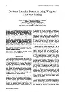
each pair of consequent features are connected together and the contained area is marked black.

100

0

(k) Png, k = 20

140

8

0.6

150

S-score

180

0.3

0 0

S-score

(j) Png, k = 8

7

50

0 0.2

6

S-score

200

0.1

5

(i) Gif, k = 28

250

Number of Samples

Number of Samples

0.3

200

0

4

0.4

0.2

21

Fig. 4.

100

250

0

27

26

22

150

S-score

50

3

0.6

28 7

0.4

2

0.8

8

19 18

(h) Gif, k = 20

100

6

32 1

0 0

(g) Gif, k = 8

150

27

29

50

0 0

30 5

0.2

20 250

0

31 4

0.8

26

24

0.6

(f) Data, k = 28

250

50

3

S-score

250

100

(c) avoid utf8 tolower 1

2

0.6

28 7

0.4

23

150

29

32 1

400

0

S-score

(d) Data, k = 8

(b) alpha upper

3

16 15 17

1 2

0.6

28

600

14 19 18

200

0 0

30 800

32 1

13 20

16 15 17

1 31

12 21

14 19 18

(a) alpha mixed

1000

22

13 20

16 15 17

(c) Shellcode, k = 28

1400

1200

Number of Samples

Number of Samples

(b) Shellcode, k = 20

1400

12 21

14 19 18

(a) Shellcode, k = 8

22

13 20

0

0.1

0.2

0.3

0.4

0.5

0.6

S−score

(n) Benign code, k = 20

0

0

0.1

0.2

0.3

0.4

0.5

0.6

S−score

(o) Benign code, k = 28

The S-score Distribution with Different k

score greater than 0.1. However, as shown in Figure 3(c), if the length of calculation window is set to 28, 3 shellcode samples have S-score with ‘null’. On the other hand, the S-score of all other samples are reduced close to 0 if k is greater than 20, as shown in Figure 3, . The results suggest that the combination of calculation window length k = 28 and threshold t = 0.1 be sufficient to identify shellcode with 97.9% accuracy and 0.82% false positive rate in our dataset. C. Attributing Encoded Shellcode We evaluate our shellcode representation and attribution analysis technique from several different aspects including visualization, correlation analysis of selected features, accuracy of attributing, and quantification of encoder strength. 1) Data Visualization: The visualization of shellcode samples could tell us the differences of shellcode generated from various engines in an intuitive way. We propose to visualize shellcode sample in BFR form with a radar chart graph, in which a circle is equally divided by 32 invisible lines. Each of these 32 lines represents an axis for each corresponding feature in BFR form, where the center of circle represents 0 and the periphery represents 1. Since, in the BFR form, a shellcode sample is represented as f ∈ Z32 , we used data scaling on all the samples in our dataset to transform each feature into the range of [0, 1]. The value of each feature is marked by a dot on its corresponding line. Then, the dots from

Figure 4 shows six radar charts of instances from six different shellcode engines. As we can notice, the shellcode generated by alpha mixed has strong similarity with the shellcode generated by alpha upper. They both generate shellcode with longer instructions (features 25 to 32). Shellcode generated by context time or fnstenv mov has more unconditional data transfer instructions than others (feature 3). fnstenv mov tends to use registers esi, edi and ebp more often (features 21, 22, and 23), while alpha mixed prefers eax, ecx, and edx (feature 17, 19, and 20). Because the data scaling is performed over the whole dataset, we could also notice that the size of black area differs significantly. The major reason behind this phenomenon is that some engines tend to generate much longer data sequence even if the input payload is the same. Obviously, the shellcode generated by call dword xor or avoid utf8 tolower is smaller than its counterpart generated by alpha mixed in size. 2) Effectiveness of Feature Selection: In order to prove our feature selection approach in BFR is effective and the extracted features are not redundant, we utilize Pearson product-moment correlation coefficient to measure the linear relationships between each pair of features in BFR form. Given two features fi and fj in BFR, the correlation coefficient ρfi ,fj is a measure of the linear dependency between them that is defined as E[(fi −µfi )(fj −µfj )] ρfi ,fj = , where µfi is the mean and σfi σfi σfj is the standard deviation of this feature value over our dataset. The maximum value for correlation coefficient, which is 1, represents a perfect positive correlation between two variables, and the minimum value -1 indicates a perfect negative correlation. If |ρfi ,fj | is close to 1, it means one of the selected features could be linearly represented by another one, hence it clearly indicates redundancy. We calculated the correlation coefficient for each pair of features over our dataset, and computed the average of their absolute values defined as ∑ |ρf ,f | P = i̸=j496 i j , where 496 is the number of feature pairs (32 × 31)/2. The result was P = 0.3428 that indicates our feature selection is not redundant.

TABLE II.

0.9 0.85

0.82

Accuracy

Accuracy

0.75 0.7

C=0.25 C=0.5 C=1 C=4 C=8 C=16 C=32

0.65 0.6 0.55 0.5 0.015625

0.03125

0.0625

0.125

0.25

0.81 0.8 0.79 0.78 0.77 0.125

0.5

0.25

0.5

(a) Radial Basis Function

2

4

8

0.4

0.85

Accuracy

0.5

0.8

C=0.0625 C=0.125 C=0.25 C=0.5 C=1

0.75

0.3 0.7 0.2

0.015625

0.03125

0.0625

0.125

Gamma

(c) Sigmoid Function

Fig. 5.

32

(b) Linear Function

C=0.0625 C=0.125 C=0.25 C=0.5 C=1

0.6

0.1 0.0078125

16

0.9

0.7

Accuracy

1

C

Gamma

0.8

0.25

T HE S TRENGTH

Engine

0.8

0.65 0.03125

0.0625

0.125

0.25

alpha mixed alpha upper avoid utf8 tolower call4 dword xor context cpuid context stat context time countdown fnstenv mov jmp call additive nonalpha nonupper shikata ga nai single static bit random data generator

Variation Strength 1.91 1.42 1.29 2.17 0.27 0.93 0.94 0.80 2.29 1.46 0.74 0.98 1.58 1.22 3.31

OF

E NCODERS

Propagation Strength 26.07 22.50 14.53 25.82 4.66 12.53 12.51 10.42 26.11 15.74 9.91 11.93 16.78 15.87 49.07

Overall Strength 49.91 31.86 18.70 55.96 1.25 11.65 11.73 8.33 59.71 22.91 7.36 11.71 26.46 19.34 162.59

0.5

Gamma

(d) Polynomial Function

Attribution Accuracy with Four Kernel Functions

3) Parameter Tuning: In the SVM model, the factors that affect the classification result include the penalty parameter C, the kernel function, and corresponding parameters in the kernel function. We randomly divided our shellcode dataset into a training set and a testing set, which is a standard approach in machine learning. The training set has 60% of samples from each class and the testing set consists of the rest of samples, 40% of samples. To find the best kernel function and parameters, we used a grid-search for possible parameter combinations on the training set to learn SVM model with four popular kernel functions [6] and to evaluate it on the testing set. Radial basis function (RBF): A RBF kernel takes the form of K(f (i) , f (j) ) = exp(−γ ∥ f (i) − f (j) ∥2 ), γ > 0. Therefore, there are two parameters to tune: the penalty parameter C and γ. We used a grid-search to test exponentially growing sequence of C = 2−3 , 2−2 , ..., 28 and γ = 2−7 , 2−6 , ..., 25 . Figure 5(a) shows the accuracy of testing when different parameter combinations are used. The results show that, when C is fixed, the best r is in the range [2−4 , ..., 2−2 ]. On the other hand, when r is fixed, the best C is above 8. We found the best (C, γ) combination (8, 0.25) with the accuracy of 85.02% in attributing testing samples to its class; Linear function: A linear function takes the form of K(f (i) , f (j) ) = f (i)T f (j) . Therefore, the only parameter for tuning is C. We tested C = 2−3 , ..., 25 and found the best penalty parameter C = 8 with 82.11% accuracy as shown in Figure 5(b); Sigmoid function: A sigmoid function takes the form of K(f (i) , f (j) ) = tanh(γf (i)T f (j) + r), γ > 0. We found the best (C, γ, r) combination (2−4 , 2−5 , −2−3 ) with the accuracy of 63.70% in attributing testing samples to its class as shown in Figure 5(c); Polynomial function: A polynomial function takes the form of K(f (i) , f (j) ) = (γf (i)T f (j) + r)d , γ > 0. We evaluated the combinations of C = 2−1 , ..., 23 , γ = 2−5 , ..., 2−1 , r = 2−3 , ..., 2−1 and d = 2, 3, 4. We found the best (C, γ, r, d) combination (4, 0.25, 0.125, 3) with the accuracy of 84.57% as shown in Figure 5(d). In summary, our results suggest that RBF, linear, and polynomial kernels be appropriate for attributing shellcode samples in terms of accuracy. However, the computation cost for each kernel is

different. We discuss the system performance using different kernels in Section IV-D. 4) The Hardness of Multi-class Attributing: We tested a radius basis function–the kernel function with the highest accuracy– with parameter combination C = 8, γ = 0.25 in subsets of our dataset to find out whether increasing the number of shellcode engines for the classification makes the problem harder to solve. We performed the same testing procedure mentioned in the previous section to test the accuracy of our model for 2, ..., 13 shellcode classes. Our model can achieve 100% classification accuracy for up to 6 shellcode engines and 95.0% classification accuracy for 11 classes, which is higher than previous efforts [16]. Note that, compared with [16] in which a specific model is built for each shellcode class, our approach only use one model to classify instances from all kinds of classes, hence does not need different parameter settings for each model. 5) The Strength of Encoding Engines: In [26], the authors introduced variation strength, propagation strength and overall strength on the byte sequence of shellcode to measure polymorphic engines’ strength. We redefine these measures to accommodate our binary representation form. Variation strength: The variation strength of an encoding shellcode engine measures the engine’s ability to generate shellcodes that span a sufficiently large portion of 32-dimensional BFR space. We make use of covariance matrix to recover the hyper-ellipsoidal bound on the of each engine. The ma∑dataset N trix is defined as Σ(e) = N1 i=1 (f (i) − µ)(f (i) − µ)T , where N is the number of samples generated by an engine e in our dataset. Σ ∈ R32×32 describes the shape of a 32-dimensional ellipsoid. Then, the problem of calculating the spanned set is transformed to an eigenvector decomposition problem. Thus, v and λ, such as Σv = vλ, are recovered∑where√λ is a 32 1 32-dimensional vector. We define Ψ(e) = 32 |λi | as i=1 the variation strength of an encoder e; Euclidean distance: Given two BFRs f (i) and f (j) which represent two samples in our dataset, the Euclidean √ distance between these BFRs ∑32 (i) (j) 2 (i) (j) is defined as δ(f , f ) = k=1 (fk − fk ) ; Propagation strength: Given N samples labeled as outputs of an engine e, the propagation strength of this engine describes the average Euclidean distance between all sample pairs defined ∑ as Φ(e) = N (N2−1) i̸=j δ(f (i) , f (j) ); Overall strength: The overall strength of an encoder e is defined as the multi-

TABLE III.

S HELLCODE ATTRIBUTION T IME C OST ( MILLISECOND )

Kernel Function Radial Basis function Linear function Sigmoid function Polynomial function 1 2

Parameter Combination C = 8, γ = 0.25 C=8 C = 2−4 , γ = 2−5 r = −2−3 C = 8, γ = 0.25 r = 0.125, d = 3

Training1 Time 2,760 1,840 15,640 3,120

Classification2 Time 1,720 1,320 7,240 1,230

Training set includes 7,906 shellcode samples Testing set includes 5,270 shellcode samples

plication of its variation strength and propagation strength Π(e) = Φ(e) × Ψ(e). The higher overall strength of an engine indicates that its shellcode instances are more obscured and harder to be correctly attributed. In order to remove the differences introduced by different payloads, we only took the shellcode instances generated by different engines from the same payload into account. Table II shows the strength of these engines based on our metrics. random data generator refers to a generator that outputs a group of randomly generated strings with the value of each byte in {0, ..., 255}. The lengths of these strings are also randomly generated with the value from 160 to 400 bytes, which is the length range of shellcode we mostly observed. It is not surprising to discover that random data generator is the strongest ‘encoder’ with the overall strength of 162.59. Among all the encoders, we also noticed that fnstenv mov and call4 dword xor are two of strongest engines based on our metrics, while context cpuid is the weakest one. alpha mixed (49.91) is stronger than alpha upper (31.86), because it could output both upper and lower case alphabets. However, the strength is not doubled because the size of output character set is doubled. Similar observation can be found between nonalpha and nonupper where nonupper shows a little bit stronger obfuscation.

D. Performance Evaluation We conducted experiments on a machine with Intel Core2 Duo CPU 3.16 GHz 3.25 GB RAM running Windows 7, IDA Pro 5.6 and Matlab R2010a. We used Windows API GetTickCount to measure the performance of our program in C language and cputime to measure the elapsed time in Matlab program. The training phase of Markov-chain-based model only took less than 15 milliseconds to learn from 140 shellcode samples. The detection phase with the calculation window length of 20 took less than a second to calculate the S-score of 1,200 data streams with variable-length from 160 bytes to 400 bytes. Table III shows the time cost for shellcode attribution in training and testing with different kernel functions. We evaluated the performance of the parameter combination with the accuracy of each kind of kernel function. Linear function is the most efficient kernel with 1,840 milliseconds in training for 7,906 samples and 1,320 milliseconds in classifying 5,270 samples. Radial basis function that has 85.02% accuracy in classifying 14 shellcode classes is also efficient, taking 2,760 milliseconds in training and 1,720 milliseconds in classification.

V.

D ISCUSSION

A. The Feasibility of Using One Model It is possible to use one unified model to detect and attribute encoded shellcode in a single step. However, we choose not to adopt such an approach due to the following issues: i) the problem of differentiating code from data and the problem of attributing detected attack are two separate issues. By separating these two research issues, we could achieve the most accurate results for each group. However, we have to balance the detection rate and attribution rate if these two problems are mixed together; ii) we only consider sequential information to detect and attribute shellcode and we use Markov-chain-based model to fulfill this requirement. In the training phase, we need to train a specific sequential model for each shellcode class instead of modeling all shellcode samples together. Correspondingly, in the detection phase, the given suspicious data stream has to be evaluated by all trained models. With the increased number of shellcode class, the evaluation process will be slow and infeasible for online detection; and iii) we also consider a standard classifier, such as SVM and neural networks, to perform detection and attribution. Most standard classifiers do not support modeling of sequential knowledge that may render valuable ‘ordering’ information useless. B. Using Opcode Functionality Sequence to Detect Shellcode In our experimental evaluation, we also considered to use opcode functionality sequence to detect shellcode instead of opcode mnemonic sequence. For a given instruction sequence i = (i1 , ..., im ), its opcode functionality sequence is represented as sT = (s1 , ..., sm ), where sk ∈ {1, ..., 10} that is the set of the opcode functionality category. While opcode mnemonic sequence maps encoded shellcode instances into a am dimensional space, opcode functionality sequence maps them into an even lower dimensional space, 10m . However, the evaluation results show that both false negative and false positive rate are high with this representation. We believe the reason is that the 10m dimensional space is not sufficient to capture the difference between code and data. C. The Arms Race and Future Work It is possible for malicious code distributors to disturb our shellcode detection method by permutating the locations of instructions in a sequence. For instance, the sequence 1: [mov eax, 1;] 2: [add eax, 1;] 3: [mov ebx, 1;] 4: [add ebx, 1] has different transition probabilities from the sequence 3; 1; 2; 4. However, their permutation choices are limited in which the semantics of the instruction sequence has to be maintained. For example, permutation to 2; 4; 3; 1 is not possible. To cope with this potential arms race, we could integrate machine code slicing [10] into our approach. The previous example could be sliced into two independent pieces 1; 2 and 3; 4, and only intra-piece transition probabilities are considered for learning and detection. In addition, higher order Markov chain may be utilized to enhance the accuracy of our approach but might need to minimize unexpected performance overhead. For the attribution part, attackers may deliberately cram garbage instructions to interfere the distribution patterns used in BFR.

Fortunately, this issue is easier to solve than byte cramming attacks with the awareness of semantics in disassembly. We could perform data flow analysis [30] on machine code first to prune useless instructions in a sequence to handle this challenge. VI.

R ELATED W ORK

Newsome et al. introduced Polygraph [24], a mechanism that is robust to generate signatures for polymorphic code. Li et al. [19] proposed Hamsa, a noise-tolerant and attackresilient network-based automated signature generation system for polymorphic worms. Approaches to generate vulnerabilitybased signatures [5], [20] were also proposed on the network level without any host-level analysis of execution. However, Chung et al. [9] showed that all of these signature generation schemes are vulnerable to advanced allergy attacks. APE [27] calculated the maximum execution length of a byte sequence, and learned threshold for detecting possible malicious packages. Stride [3] complemented the previous effort by adding new criteria including non-privileged instruction in a byte sequence to identify sled in shellcode. Chinchani et al. [7] and Kruegel et al. [17] proposed to utilize the control and data flow information in binary to detect polymorphic code. Wang et al. [30] first used data flow anomaly to prune useless instructions then compared the number of useful instructions with a certain threshold to determine if it has any code. Wang et al. [28] compared the byte frequency of normal network packages with malicious ones to figure out the byte patterns that could lead to attack detection. However, their solutions were vulnerable to byte cramming [12] and polymorphic blending attacks [13]. Recently, Kong et al. [16] proposed to take advantage of semantic analysis and sequential models on n-gram data bytes to analyze the attribution of exploits. Wartell et al. [31] developed machine learning-based algorithms to differentiate code from data. Rosenblum et al. [25] proposed to use conditional random field to extract compiler provenance from code. While most of these work focus on the byte patterns identified in binary code, Song et al. [26] presented quantitative analysis of the byte strength of polymorphic shellcode and claimed that modeling the byte patterns in shellcode is infeasible. Besides the aforementioned research efforts, several new binary encoding schemes were proposed in recent years. Mason et al. [22] proposed English shellcode engine that transforms arbitrary shellcode to a representation that is similar to English prose. Wu et al. [32] proposed mimimorphism to transform binary into mimicry counterpart that exhibits high similarity to benign programs in terms of statistical properties and semantic characteristics. VII.

for shellcode attribution. Our experiments showed that our approach does not require any signature and is only based on static analysis and supervised machine learning. The evaluation results also suggested that our solution detect and attribute shellcode to its originating engines with high accuracy and lower false positive rate.

C ONCLUSION

In this paper, we proposed a technique for modeling shellcode detection and attribution through a novel feature extraction method, called instruction sequence abstraction, that extracts distinguishable features from suspicious data stream by reducing the size of input data dimension and removing ambiguous byte patterns. We also presented a Markov-chain-based model for shellcode detection and adopted support vector machines

ACKNOWLEDGEMENT This work was partially supported by the grants from National Science Foundation and Department of Energy. R EFERENCES [1] IDA Pro Disassembler. http://www.datarescue.com/idabase. [2] Intel 8086 family user’s manual octobe 1979. http://matthieu.benoit.free.fr/cross/data-sheets/8086-family-usersmanual.pdf. [3] P. Akritidis, E. Markatos, M. Polychronakis, and K. Anagnostakis. Stride: Polymorphic sled detection through instruction sequence analysis. In SEC’05, pages 375–391. [4] B. Boser, I. Guyon, and V. Vapnik. A training algorithm for optimal margin classifiers. In Proc. COLT, pages 144–152, 1992. [5] D. Brumley, J. Newsome, D. Song, H. Wang, and S. Jha. Towards automatic generation of vulnerability-based signatures. In S&P’06. [6] C.-C. Chang and C.-J. Lin. LIBSVM: A library for support vector machines. ACM TIST, 2:27:1–27:27, 2011. [7] R. Chinchani and E. Van Den Berg. A fast static analysis approach to detect exploit code inside network flows. In RAID’06, pages 284–308. [8] M. Christodorescu, S. Jha, S. Seshia, D. Song, and R. Bryant. Semanticsaware malware detection. In S&P’05, pages 32–46. [9] S. Chung and A. Mok. Advanced allergy attacks: Does a corpus really help? In RAID’07, pages 236–255. [10] C. Cifuentes and A. Fraboulet. Intraprocedural static slicing of binary executables. In Software Maintenance’97, pages 188–195. [11] C. Cortes and V. Vapnik. Support-vector networks. Machine learning, 20(3):273–297, 1995. [12] T. Detristan. Polymorphic shellcode engine using spectrum analysis. In Phrack Magazine, 2003. [13] P. Fogla, M. Sharif, R. Perdisci, O. Kolesnikov, and W. Lee. Polymorphic blending attacks. In USENIX Security’06, pages 241–256, 2006. [14] R. Horspool and N. Marovac. An approach to the problem of detranslation of computer programs. The Computer Journal, 23(3):223, 1980. [15] J. Kolter and M. Maloof. Learning to detect and classify malicious executables in the wild. The Journal of Machine Learning Research, 7:2721–2744, 2006. [16] D. Kong, D. Tian, P. Liu, and D. Wu. Sa3: Automatic semantic aware attribution analysis of remote exploits. In SECURECOMM’11, pages 1–19. [17] C. Kruegel, E. Kirda, D. Mutz, W. Robertson, and G. Vigna. Polymorphic worm detection using structural information of executables. In RAID’06, pages 207–226, 2006. [18] W. Landi. Undecidability of static analysis. ACM LOPLAS, 1(4):323– 337, 1992. [19] Z. Li, M. Sanghi, Y. Chen, M. Kao, and B. Chavez. Hamsa: Fast signature generation for zero-day polymorphicworms with provable attack resilience. In S&P’06. [20] Z. Li, L. Wang, Y. Chen, and Z. Fu. Network-based and attack-resilient length signature generation for zero-day polymorphic worms. In ICNP, pages 164–173, 2007. [21] C. Linn and S. Debray. Obfuscation of executable code to improve resistance to static disassembly. In Proc. CCS, pages 290–299, 2003. [22] J. Mason, S. Small, F. Monrose, and G. MacManus. English shellcode. In CCS’09, pages 524–533. [23] H. Moore. The metasploit project. http://www.metasploit.com/, 2009. [24] J. Newsome, B. Karp, and D. Song. Polygraph: Automatically generating signatures for polymorphic worms. In S&P’05, pages 226–241. [25] N. Rosenblum, B. Miller, and X. Zhu. Extracting compiler provenance from program binaries. In Proc. PASTE, pages 21–28, 2010. [26] Y. Song, M. Locasto, A. Stavrou, A. Keromytis, and S. Stolfo. On the infeasibility of modeling polymorphic shellcode. In CCS’07, pages 541–551. [27] T. Toth and C. Kruegel. Accurate buffer overflow detection via abstract payload execution. In RAID’02, pages 274–291. [28] K. Wang, G. Cretu, and S. Stolfo. Anomalous payload-based worm detection and signature generation. In RAID’06, pages 227–246. [29] X. Wang, Y. Jhi, S. Zhu, and P. Liu. Still: Exploit code detection via static taint and initialization analyses. In ACSAC’08, pages 289–298. [30] X. Wang, C. Pan, P. Liu, and S. Zhu. Sigfree: a signature-free buffer overflow attack blocker. In USENIX Security’06. [31] R. Wartell, Y. Zhou, K. Hamlen, M. Kantarcioglu, and B. Thuraisingham. Differentiating code from data in x86 binaries. In Proc. PKDD, pages 522–536, 2011. [32] Z. Wu, S. Gianvecchio, M. Xie, and H. Wang. Mimimorphism: a new approach to binary code obfuscation. In CCS’10, pages 536–546.