Using JCP format

JOURNAL OF CHEMICAL PHYSICS

VOLUME 113, NUMBER 16

22 OCTOBER 2000

Thermal conductivity of diamond and related materials from molecular dynamics simulations Jianwei Che, Tahir C ¸ ag˘ın, Weiqiao Deng, and William A. Goddard IIIa) Materials and Process Simulation Center, Beckman Institute, Division of Chemistry and Chemical Engineering, California Institute of Technology, Pasadena, California 91125

共Received 25 January 2000; accepted 25 July 2000兲 Based on the Green–Kubo relation from linear response theory, we calculated the thermal current autocorrelation functions from classical molecular dynamics 共MD兲 simulations. We examined the role of quantum corrections to the classical thermal conduction and concluded that these effects are small for fairly harmonic systems such as diamond. We then used the classical MD to extract thermal conductivities for bulk crystalline systems. We find that 共at 300 K兲 12C isotopically pure perfect diamond has a thermal conductivity 45% higher than natural 共1.1% 13C兲 diamond. This agrees well with experiment, which shows a 40%–50% increase. We find that vacancies dramatically decrease the thermal conductivity, and that it can be described by a reciprocal relation ␣ with a scaling as n ⫺ v , with ␣ ⫽0.69⫾0.11 in agreement with phenomenological theory ( ␣ ⫽1/2 to 3/4兲. Such calculations of thermal conductivity may become important for describing nanoscale devices. As a first step in studying such systems, we examined the mass effects on the thermal conductivity of compound systems, finding that the layered system has a lower conductivity than the uniform system. © 2000 American Institute of Physics. 关S0021-9606共00兲70140-1兴

wires; Balandin and Weng6 calculated the thermal conductivity reduction in the Si quantum well; Gurevich7 discussed in detail the use of general principles of physical kinetics to describe phonon transport theory. These approaches must assume the fundamental constitutive equation and parameters. The advantage of using the Boltzmann equation 共BE兲 is that large systems can be studied reasonably quickly. However, certain parameters such as phonon relaxation time ␶ ( ␻ ) and phonon density of states 共DOS兲 must be obtained either from experiments or other theoretical estimates. In addition, solving the integro-differential BE for general cases is nontrivial. Moreover, for nanoscale electronic devices, it is very difficult to measure directly phonon properties required to predict the thermal conductivity. Thus, it is of great interest to develop methods for using first principles atomistic simulations to predict the thermal properties. In particular, recent advances in characterizing the interactions between atoms using classical force fields 共FF兲 based on high level quantum mechanical calculations provide the opportunity to make first principles predictions on interesting organic and inorganic materials without additional data from experiment. This also allows the effect of microscopic structure 共interfaces and surface reconstruction兲 to be studied quantitatively. In addition, such atomistic simulations can provide the input data 共the DOS and relaxation times兲 to the BE approach. Thus, it can bridge between atomistic dynamics and continuum kinetics. One can generally partition the thermal conductivity of a material into

I. INTRODUCTION

As the dimensions of electronic and mechanical devices are shrunk into nanometer dimensions, the thermal conductivity becomes quite important since functioning electronic, piezoelectric, and thermogalvanic devices may require that significant energy be dissipated in a small region. However, the experimental measurement of thermal conductivity1 becomes quite difficult for nanometer scale devices, particularly for the complex geometries of real devices. Consequently, it is of interest to develop reliable theoretical and computational methods for predicting the thermal properties of nanoscale materials and devices. There are two major approaches to theoretical studies of the thermal conductivities of materials. 共1兲 The most fundamental approach is to base the calculations on first principles atomistic simulations. This allows the properties for new materials to be predicted in advance of experiment. This is particularly useful for nanoscale devices where the experiments are quite difficult. Atomistic simulations have been employed to determine diffusion coefficients, viscosities, and thermal conductivities for fluids. Both equilibrium and nonequilibrium dynamic simulations2–4 have been reported for various systems. The calculated results are often in reasonable agreement with experimental measurements. 共2兲 More commonly, thermal conductivity has been studied using continuum models and kinetic theories such as the Boltzmann transport equation. For example, Walkauskas et al.5 calculated the lattice thermal conductivity of GaAs

共1兲 the electronic thermal conductivity, which depends on the electronic band structure, electron scattering, and electron–phonon interaction, and

a兲

Author to whom all correspondence should be addressed; electronic mail: [email protected]

0021-9606/2000/113(16)/6888/13/$17.00

6888

© 2000 American Institute of Physics

Downloaded 02 Mar 2004 to 131.215.16.37. Redistribution subject to AIP license or copyright, see http://jcp.aip.org/jcp/copyright.jsp

J. Chem. Phys., Vol. 113, No. 16, 22 October 2000

共2兲 the lattice conductivity, which depends mainly on the phonons 共nuclear vibrations兲 and phonon scattering. In this paper, we only consider the lattice thermal conductivity 共as derived from the FF兲. This is appropriate for the systems considered here since they have large band gaps leading to small electronic contributions to thermal conduction. Because the phonon main free path in crystalline solids is much longer than that in liquids and amorphous solids, it is particularly challenging to calculate thermal conductivity for solid phase crystalline systems. Thus, to simulate the total phonon transport properties, one might expect that the periodic cell for the molecular dynamics 共MD兲 simulations should be larger than the phonon mean free path, which can be on the order of hundreds nanometers. Moreover, calculating the phonon–phonon interactions responsible for limiting the thermal conductivity is one of the most complicated problems in solid physics. Indeed, there have been few attempts to achieve this objective 共Gillan8 reviewed calculation of ionic solids by MD, Paolini9 calculated the thermal conductivity of defective ionic crystals, Li, Porter, and Yip10 studied thermal conductivity of crystalline ␤-SiC using atomistic simulations, Murashov11 calculated the thermal conductivity of model zeolites via MD. Recently, Volz and Chen12–14 extensively investigated thermal conductivity of silicon crystals and silicon nanowires using MD and BE兲. We examine herein how to use MD simulations to provide some understanding of the various processes related to thermal conductivity and discuss the limitations in such approaches. We use the Green–Kubo 共GK兲 relation derived from linear response theory to extract the thermal conductivity from energy current correlation functions. We find that the accuracy of thermal conductivity is sensitive to the size of the periodic unit cell in the MD simulation 共which limits the phonon wavelength兲. However, we find that it is possible to extract an accurate thermal conductivity from periodic cells 60 times smaller than the actual phonon mean free path. The reason is that the energy current correlation time is much shorter than energy relaxation time. We illustrate this by using equilibrium MD simulations to calculate thermal conductivity of bulk crystalline diamond, including the effect on vacancies, isotopes, mass, and nanostructures. Since diamond is well known as an exceedingly good thermal conductor, these calculations on diamond crystal provide a rigorous test of our methods. Section II outlines the theoretical background for thermal conductivity calculation. Section III provides the simulation details and the form of the FF. Section IV gives numerical results along with analysis and discussions. Finally, Sec. V summarizes the paper.

II. THEORETICAL BACKGROUND

Thermal conductivity of diamond from simulations

Jជ q ⫽⫺⌳•ⵜT,

共1兲

where ⌳ is the thermal conductivity tensor and Jជ q is the heat current produced by the temperature gradient ⵜT. In energy conservation relation, the total energy current Jជ E includes both the heat current Jជ q plus the convection contribution, ␮ J, where Jជ is the particle current, and ␮ is the chemical potential. The relation between energy current and heat current is given by16 Jជ q ⫽Jជ E ⫺ ␮ Jជ .

共2兲

We will consider solids, where diffusion is negligible. In the classical limit, the energy density h(rជ ) reduces to the site energy of each particle. Therefore, heat currents can be expressed in terms of local classical properties of each particle R⫽

兺i rជ i h i ,

共3兲

H⫽

兺i h i ,

共4兲

d R. dt

共5兲

Jជ q ⫽

One approach to the simulation would be to put the system in contact with two different reservoirs with temperature T 1 and T 2 . The heat current would be calculated when the system arrives at the steady state. However, with 106 atoms in a unit cell, the system will only have dimensions of ⬃25 nm on a side. Thus, even a small temperature difference of 10 K across this system would have a thermal gradient of 4⫻108 K/m, an unrealistically huge thermal loading for a macroscopic system. It is unlikely that linear response theory will still hold under such extreme thermal loading. Moreover, even this temperature gradient may be smaller than the thermal fluctuations in the system, making it difficult to obtain converged results in reasonable simulation times. Instead, we use the fluctuation–dissipation theorem from linear response theory to provide the connection between the energy dissipation in irreversible processes and the thermal fluctuations in equilibrium.15 In this case, the thermal conductivity tensor can be expressed in terms of heat current correlation functions,15,16 ⌳⫽

1 k BT 2V

冕

⬁

0

dt C qJ 共 t 兲 ,

C qJ 共 t 兲 ⫽ 具 Jជ q 共 t 兲 ;Jជ q 共 0 兲典 ,

共6兲共7兲

where C qJ is the quantum canonical correlation function, defined as15

A. Fourier’s law and the Green–Kubo relation

The macroscopic thermal conductivity is defined from Fourier’s law for heat flow under nonuniform temperature distribution. The steady state heat flow Jជ q is obtained by keeping the system and reservoirs in contact,

6889

具 a;b 典 ⫽

1 ␤

冕

␤

0

d ␰ Tr关 ␳ exp共 ␰ H 兲 a exp共 ⫺ ␰ H 兲 b 兴 ,

共8兲

where ␳ is the density matrix of the system at equilibrium, ␤ ⫽ 1/k B T, and a,b are dynamic operators.


6890

Che et al.


Substituting Eq. 共17兲 into Eq. 共6兲, leads to

B. Classical limits and the semiclassical approximation

⌳⫽⌳c⫹

1. The classical limit

Equation 共7兲 is a quantum mechanical correlation function, which is difficult to evaluate directly in general. In this section, we discuss the classical limit of Eq. 共7兲 and a semiclassical implementation. In the classical limit, ប→0, the canonical correlation function 共10兲 reduces to the classical correlation function, C cJ 共 t 兲 ⫽ 具 Jជ q 共 t 兲 Jជ q 共 0 兲典 ,

共9兲

where C cJ (t) is obtained by phase space averaging,

具a b典⫽

兰 d⌫ exp共 ⫺ ␤ H 兲 a b . 兰 d⌫ exp共 ⫺ ␤ H 兲

共10兲

共Note that both classical and canonical correlation functions are even functions.兲 Using Eq. 共9兲 we obtain the thermal conductivity as ⌳c ⫽

冕

1 k BT 2V

⬁

0

共11兲

dt C cJ 共 t 兲 .

Usually, quantum effects are not very crucial when T ⰇT D , where T D is the Debye temperature. Unfortunately, the Debye temperature of diamond17,18 is ⬃1840– 2000 K, far too large to simply neglect quantum effects. 2. Quantum corrections

To investigate the quantum corrections, we first introduce the one-side quantum correlation function of heat cur⫺ rent, C ⫹ J (t) and C J (t),

ជ ជ C⫹ J 共 t 兲 ⫽Tr关 ␳ J q 共 t 兲 J q 共 0 兲兴 ,

共12兲

ជ ជ C⫺ J 共 t 兲 ⫽Tr关 ␳ J q 共 0 兲 J q 共 t 兲兴 . 19

It can be proved

that

C⫹ J

and

共13兲 C⫺ J

共14兲

Using Eq. 共14兲 in Eq. 共7兲 leads to 1 ␤

冕

␤

0

d␰ C⫹ J 共 t⫹i ␰ ប 兲 .

共15兲

In order to estimate the quantum correction to the classical equation, Eq. 共11兲, we need to find a relationship between the quantum canonical correlation function and its classical counterpart. Several authors have suggested methods that approximately map classical correlation functions to quantum ones. Schofield20,21 suggested

冉

C ⫹ 共 t 兲 ⫽C c t⫺

冊

iប ␤ , 2

共16兲

which satisfies the detailed balance requirement. Using Eq. 共16兲, we can expand the right-hand side into power series of ប, C q⫹ 共 t 兲 ⫽C c 共 t 兲 ⫺

共18兲

where ⌳c is obtained from Eq. 共11兲. However, due to the time reversal symmetry of the classical correlation function, the second term is zero. Similarly, the higher order terms are zero. Therefore, if Eq. 共16兲 is adopted, the quantum thermal conductivity is the same as the classical counterpart. Egelstaff22 also suggested a somewhat similar but more complex approximation. In addition, there have been some attempts to calculate quantum correlation functions from path integral and semiclassical approaches. The approximation by Egelstaff is C ⫹ 共 t 兲 ⫽C c 共冑t 2 ⫺iប ␤ t 兲 ,

共19兲

which leads to a slightly different relationship between the classical and quantum descriptions of thermal conductivity. Rather than Eq. 共18兲, we obtain ⌳⫽⌳c⫹

ប 2␤ 2 12k B T 2 V

冕

⬁

dt

0

C˙ c 共 t 兲 ⫹o 共 ប 4 兲 . t

共20兲

The second term on the right-hand side appears to be a correction to the classical thermal conductivity. However, our simulation results 共Sec. IV兲 indicate that the correction term for diamond in Eq. 共20兲 is six orders of magnitude smaller than the leading term ⌳c. We should note that neither Eq. 共16兲 nor Eq. 共19兲 is exact. Thus, it is reasonable that they lead to slightly different answers. However, we will see that the difference between them is negligible, giving us confidence in the reliability of the classical description. In Sec. II B 3, we will take a closer look at the mapping relations from the perspective of harmonic analysis.

satisfy

⫺ C⫹ J 共 t 兲 ⫽ 关 C J 共 t 兲兴 * .

C qJ 共 t 兲 ⫽

ប 2␤ 2 ˙ c 共 0 兲 ⫹o 共 ប 4 兲 , C 24k B T 2 V

iប ␤ ˙ c ប 2␤ 2 ¨ c C 共 t 兲⫺ C 共 t 兲 ⫹o 共 ប 3 兲 . 2 8

共17兲

3. Harmonic analysis

Here, we employ a harmonic analysis to examine the quantum correlations. First, we partition the quantum correlation function into the real and imaginary parts, C ⫹ 共 t 兲 ⫽C ⬘ 共 t 兲 ⫹iC ⬙ 共 t 兲 ,

共21兲

with C ⬘ 共 t 兲 ⫽ 21 关具 O 共 t 兲 O 共 0 兲典 ⫹ 具 O 共 0 兲 O 共 t 兲典兴 ,

共22兲

i C ⬙ 共 t 兲 ⫽⫺ 关具 O 共 t 兲 O 共 0 兲典 ⫺ 具 O 共 0 兲 O 共 t 兲典兴 . 2

共23兲

where O is a dynamic operator, and 具典 denotes the canonical averaging. C ⬘ (t) is an even real function, while C ⬙ (t) is an odd real function. To relate the canonical correlation function to the one side quantum correlation function, we use the Fourier transform of Eq. 共15兲, ˜ qJ 共 ␻ 兲 ⫽ C

1 ˜⫹ 关 exp共 ␤ ប ␻ 兲 ⫺1 兴 C J 共 ␻ 兲. ␤ប␻

共24兲




˜ ⫹( ␻ ) From the detailed balance relation19, C ⫺ ˜ (␻), we can express Eq. 共24兲 in terms of the ⫽exp(⫺␤ប␻)C ˜ real function C ⬘ ( ␻ ), ˜ qJ 共 ␻ 兲 ⫽ C

␤ប␻ 2 ˜C ⬘ 共 ␻ 兲 . tanh ␤ប␻ 2

共25兲

To further investigate the relationship between quantum and classical thermal conductivity, we generalize the definition of the static thermal conductivity by introducing the frequency-dependent thermal conductivity, ⌳( ␻ ), ⌳共 ␻ 兲 ⫽ ⫽

1 2k B T 2 V

冕

⬁

⫺⬁

C qJ 共 t 兲 e i ␻ t dt,

1 ˜C q 共 ␻ 兲 . 2k B T 2 V J

共26兲

Substituting Eq. 共24兲 into Eq. 共26兲, leads to ⌳共 ␻ 兲 ⫽

␤ប␻ 1 2 ˜C ⬘ 共 ␻ 兲 . tanh 2 2k B T V ␤ ប ␻ 2

共27兲

Up to this point, no approximation to the correlation functions have been made. All these equations are exact. 4. Harmonic limits

For harmonic systems bilinearly coupled to a harmonic reservoir, the real part of the quantum correlation function has a simple relation with its classical counterpart in the frequency space,23

␤ប␻ ␤ប␻ c 1 ⫹ ˜ ⬘共 ␻ 兲 ⫽ 关 C ˜ 共 ␻ 兲 ⫹C ˜ ⫺ 共 ␻ 兲兴 ⫽ ˜C 共 ␻ 兲 . coth C 2 2 2 共28兲 Similarly, the imaginary part connects with the classical correlation function via ˜ ⬙共 ␻ 兲 ⫽ C

␤ប␻ c ˜C 共 ␻ 兲 . 2

共29兲

Using Eq. 共28兲 in Eq. 共27兲, leads to ⌳共 ␻ 兲 ⫽

1 ˜C c 共 ␻ 兲 . 2k B T 2 V J

共30兲

A similar result is obtained for vibrational relaxation,23 where both the full quantum relaxation rate and full classical relaxation rate are the same for harmonic systems. Fundamentally, the finite thermal conductivity arises from the coupling strength among system vibrational modes. The processes involved in such a harmonic system are related to those in vibrational relaxation. This explains the underlying reason for the higher order terms in Eq. 共18兲 to be zero. Unfortunately, real systems are not exactly harmonic. The higher order terms in the Taylor expansion of the potential surface will contribute to the coupling of phonon modes. These anharmonicities are essential to explain in many physical phenomena in solids, including thermal conductivity. Because of anharmonicity, phonons can be created, destroyed, or scattered, leading to a finite phonon mean free path and finite thermal conductivity. The magnitude of these anharmonic effects depends on the material properties 共the interactions and structure兲. Since an accurate FF will generally account for anharmonic effects, we may use MD to study thermal conductivity. Such MD simulations implicitly include the vibrational mode couplings. Many processes involved in thermal conductivity such as boundary scattering, crystal imperfections, and isotope effects can all be included in MD simulations, although they are modeled classically. Equation 共27兲 suggests that we now need only to find a method to map the classical correlation functions into the quantum counterparts. Although Eq. 共28兲 is only exact for harmonic systems, we can still use it to approximate the quantum correlation. Since the classical counterpart already includes anharmonic behavior, the approximate quantum correlation function will also have anharmonicity partially included. ˜ c ( ␻ ) in Eq. Cao and Voth24 suggested that replacing C 共28兲 by a classical correlation function calculated from centroid potential surface provides a much better approximation for the quantum correlation function. The details on how to obtain the centroid potential surface are beyond the scope of this paper. Nevertheless, we can still estimate roughly the first-order quantum correction by considering the leading quantum correction term to the pure classical potential,25 V q 共兵 r i 其兲 ⫽V 共兵 r i 其兲 ⫹⌬V 共兵 r i 其兲 ,

This leads to the classical thermal conductivity as ⌳共 0 兲 ⫽⌳c ,

共31兲

which is exactly Eq. 共18兲. This result can be understood as follows: Equation 共28兲 is only exact for harmonic oscillators. For a purely harmonic system each normal mode is uncoupled with others. In other words, phonon modes do not interact with one another. Therefore, the only contribution to the thermal resistance for a macroscopic harmonic system is from phonon modes with wavelengths comparable to or longer than the macroscopic length scale 共where boundary scattering can couple these modes兲. This leads to the zero frequency mode condition in Eq. 共26兲. Since no ប is involved in Eq. 共30兲, this result is exact for harmonic systems. Therefore, the pure classical results are exactly the same as quantum results for harmonic systems; no quantum correction is needed.

6891

ប 2␤ ⌬V 共兵 r i 其兲 ⫽ 24

兺i

共32兲

1 ⳵ 2V , m i ⳵ 2r i

where V q is the quantum modified potential surface, and

兵 r i 其 ,i⫽1,...,3N denotes the particle coordinates. The second

term in Eq. 共32兲 modifies the interactions in the MD simulation to partially include some quantum effects. It is obvious that the new potential has a less shallow well and a lower barrier than the original classical potential. This can be understood as partially accounting for zero point energy and tunneling effects. Of course, at high temperatures the modified potential becomes the same as the classical potential. To estimate the correction to the classical correlation functions from the modified potential, we can expand the interaction potential in Eq. 共32兲 to the first order in the density matrix,


6892

Che et al.


C cq 共 t 兲 ⫽Tr关 exp共 ⫺ ␤ H⫺ ␤ ⌬V 兲 Jជ q 共 t 兲 Jជ q 共 0 兲兴 /

III. SIMULATION DETAILS A. The force field

Tr关 exp共 ⫺ ␤ H⫺ ␤ ⌬V 兲兴 ⫽C cJ 共 t 兲 ⫺ ␤ 关具 ⌬VJជ q 共 t 兲 Jជ q 共 0 兲典 c ⫺C cJ 共 t 兲具 ⌬V 典 c 兴 ⫹o 关共 ␤ ⌬V 兲 2 兴 ,

共33兲

where 具典 c indicates phase space averaging over the classical density matrix, and C cq (t) is the classical correlation function on the modified potential with the first-order quantum cor˜ cJ ( ␻ ) in Eq. 共30兲 by the Fourier transrection. Replacing C c form of C q (t), we then have the first-order quantum correction, ⌳共 0 兲 ⬇⌳c ⫺ ␤

冋

1 k BT 2V

册

冕

⬁

0

dt 具 ⌬VJជ q 共 t 兲 Jជ q 共 0 兲典 c

⫺⌳c 具 ⌬V 典 c .

3Nk B T MD⫽

冕

0

d ␻ D 共 ␻ 兲 n 共 ␻ ,T 兲 ប ␻ .

V tot⫽ ⫽

¯ i j V A 共 r i j 兲兴 , 关 V R 共 r i j 兲 ⫺B 兺i 兺 j⬎i Vij , 兺i 兺 j⬎i

共34兲 V A共 r i j 兲 ⫽ f i j共 r i j 兲

共35兲

In order to use the above-mentioned approximation, however, extra calculations have to be performed to obtain the phonon density of states, D( ␻ ), and the Debye frequency, ␻ D . The low frequency density of states, responsible for heat transport, are not trivial to calculate accurately. More important, Eq. 共35兲 tends to overestimate T MD because of the contribution from high frequencies in the spectrum that are insignificant for heat transport. In other words, the phonon modes that are most important for thermal conduction are those with very low frequencies 关i.e., Eq. 共25兲兴, and these modes are nearly classical. Therefore, we argue that Eq. 共35兲 usually is not necessary for thermal conductivity calculations, although it is important for calculating heat capacity where high frequency modes contribute significantly.10 This conclusion is consistent with Eqs. 共18兲, 共20兲, 共31兲, and 共34兲. In fact, the correct quantum heat capacity can also be derived from Eq. 共28兲 through velocity correlation functions.

共36兲

where V R and V A are the repulsive and attractive part of the pairwise binding potential, respectively. They have the same form as a general Morse potential,26 V R共 r i j 兲 ⫽ f i j共 r i j 兲

In a harmonic system, ⌬V is constant for each vibrational mode in the normal mode space. In this case, the second term in Eq. 共34兲 and all the higher order terms vanish, as expected. In this section, we have discussed the relationship between the classical lattice thermal conductivity and its quantum counterpart. The corrections to the classical thermal conductivity due to quantum effects are discussed based on the quantum corrections to the fundamental heat correlation functions. This provides insight for the role that quantum effects play in lattice thermal conductivity, and it also shows the fundamental reason why classical simulations can often capture correct thermal conductivities in many cases. In addition to the quantum corrections made to the fundamental quantities 共i.e., heat correlation functions兲, another simpler but less rigorous temperature scaling method has been used to qualitatively include quantum effects,12,14 ␻D

For the illustrative calculations in this paper, we use the Brenner bond-order-dependent FF. This FF can be written formally as summation of pairwise interactions,26

D ei j S i j S i j ⫺1 D ei j S i j S i j ⫺1

exp关 ⫺ 冑2S i j ␤ i j 共 r i j ⫺R ei j 兲兴 ,

冋冑

exp ⫺

册

2 ␤ 共 r ⫺R ei j 兲 , Sij ij ij

共37兲

共38兲

where

f i j共 r 兲⫽

冦

再冋 1⫹cos

1,

␲ 共 r⫺R (1) ij 兲 (1) R (2) i j ⫺R i j

册冎

r⭐R (1) ij (1) (2) /2, R i j ⬍r⬍R i j

0,

r⭓R (2) ij .

共39兲

f i j (r) is a cutoff function that explicitly restricts the interaction within the nearest neighbors. The bond order parameter ¯B i j depends on the environment around atoms i and j and is written as26 ¯B i j ⫽

B i j ⫹B ji C conj ⫹F i j 共 N H i 共 t 兲 ,N j 共 t 兲 ,N i j 兲 , 2

共40兲

In Eq. 共40兲, B i j implicitly contains many-body information. The detailed formulation and all parameters are given by Brenner.26

B. The heat flux

As indicated in Eq. 共36兲, the interaction potential is formally pairwise, allowing the site energy h i in Eq. 共3兲 to be defined as h i⫽

p 2i 2m i

⫹

1 2

兺j V i j .

共41兲

Therefore, the heat current can be calculated through Eq. 共5兲. Because V i j is in fact a many-body potential,20 the calculation of heat current Jជ q (t) is much more complicated than for a truly pairwise FF. After some algebra steps, Jជ q is given by Jជ q 共 t 兲 ⫽

1

兺i vជ i h i ⫹ 2 兺兺 rជ ik Fជ kli j • vជ i , i, j k,l

共42兲

with




6893

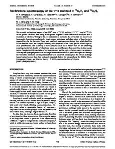
FIG. 1. The heat current correlation function and the double exponential fitting for the N⫽4096 atom simulation of 12C diamond (T⫽300 K, t run⫽400 ps. The insets show the short time region at different scales. The parameters for the fitted double exponential function 共dashed lines兲 are given in Table I.

ជ kl F i j ⫽⫺

⳵ V kl . ⳵ rជ i j

共43兲

In deriving Eqs. 共42兲 and 共43兲, we implicitly imposed the condition that there is no net momentum for the system. For a truly pairwise FF, Eq. 共42兲 recasts to the familiar form15,27 Jជ q 共 t 兲 ⫽

1

ជ i j • vជ i . rជ i j F 兺i vជ i h i ⫹ 2 兺 i, j

共44兲

C. Dynamic systems

A 1 fs time step was employed in all MD simulations. For each system, we initially equilibrated the system using Gaussian thermostat MD 共300 K兲 for 40 ps. After equilibration, we carried out 400 ps of constant energy (NVE) MD, calculating the heat current for every time step. All simulations on diamond started with a cubic unit cell constant of 3.556 Å. This unit cell was extended to build large supercells for the MD simulations 共thus, an 8⫻8⫻8 cell leads to 4096 atoms兲. Periodic boundary conditions were applied to the super cell in all three directions. IV. NUMERICAL RESULTS AND ANALYSIS A. Bulk diamond, isotopically pure

To test the convergence of MD simulations on thermal conductivity, we carried out simulations for cubic diamond, described with supercells containing 512 (4⫻4⫻4), 1000 (5⫻5⫻5), 1728 (6⫻6⫻6), 2744 (7⫻7⫻7), 4096 (8 ⫻8⫻8), and 8000 (10⫻10⫻10) atoms. Since diamond is isotopic, we used the scalar thermal conductivity that is the average value of three principle directions 共which reduces the uncertainty in the theoretical values兲. As discussed in previous sections, the phonon mean free path is the limiting factor to obtaining accurate results. For too small a simulation cell, the time for phonon to travel through the simulation cell is much shorter than the decay time of the current correlation function. This causes the phonons to be scattered

more frequently than they would be in the infinite system. In this case, only the short time correlation function is accurate. Even so we can estimate the thermal conductivity from simulations using periodic cells smaller than the mean free path. Thus, based on the macroscopic law of relaxation and Onsager’s postulate for microscopic thermal fluctuation, we expect that the asymptotic decay of the heat correlation function will be exponential. Since the kinetic coefficients depend mostly on long time decay rate behavior and since an exponential-decay behavior is exhibited in a microscopic time scale, we expect that a medium-sized simulation cell can be used to extract the decay rate of the heat dissipation. Figure 1 shows the heat current correlation functions at short times for a cubic diamond crystal with 4096 atoms. We see a rapid initial decay (⬃50 fs) followed by a long time exponential decay of the correlation function. Probably the initial fast decay is due to high frequency optical modes in the crystal, which do not significantly contribute to thermal conductivities 共either conceptually and computationally兲, because they couple only weakly to the low frequency acoustic modes and they are little populated at room temperature. To fit the correlation function we used a double exponential function C cJ 共 t 兲 ⫽A o exp共 ⫺t/ ␶ o 兲 ⫹A a exp共 ⫺t/ ␶ a 兲 ,

t⭓0,

共45兲

where the subscripts o and a denote fast optical modes and slow acoustic modes, respectively. The thermal conductivity is then given by ␭⫽

1 共 A ␶ ⫹A a ␶ a 兲 . k BT 2V o o

共46兲

The parameters A o , ␶ o ,A a , and ␶ a , are derived from the first 3 ps using nonlinear least-squares methods 共Mazquazlt– Levenberg兲. This leads to the results in Table I, where we see that high frequency optical modes contribute only 0.1% to the thermal conductivity. Note that the current correlation function at very short time (⭐20 fs) is not exponential in the


6894

Che et al.


TABLE I. Parameters for the double exponential fitting of the heat current correlation functions for 12C diamond based on Eq. 共45兲. A o /V ⫽810.5 共kcal/mol兲2/共Å ps2兲 and A a /V⫽189.6 共kcal/mol兲2/共Å ps2兲. Atoms

A o /V

␶ o (ps)

A a /V

␶ a (ps)

512 1000 1728 2744 4096 8000 ⬁

822.0 805.3 813.6 814.7 811.0 808.1 810.5

0.005 75 0.005 92 0.005 77 0.005 75 0.005 71 0.005 82 0.005 8

138.9 147.2 198.0 181.8 233.9 176.3 189.6

10.605 10.608 16.393 14.719 16.527 16.656 16.66

strict sense, since only Markovian processes have an exponential decay correlation function. In most physical processes, nonexponential decay of the correlation function near t⫽0 is quite common. However, for the cases studied here, this does not make a significant difference in the final calculated thermal conductivity. Therefore, it is satisfactory to use an exponential function to fit the initial trend. 共This is the cause of the fitting function overshooting the value at the origin.兲 Figure 2 shows the dependence of the calculated thermal conductivities on the size of the simulation cell. The uncertainties shown here are estimated by 冑2 ␶ /t run where t run is the simulation length. When the simulation cell is too small, the particles in the simulation cell do not have sufficient time to lose their previous dynamic information before a periodically equivalent phonon travels to the same place. As a result the longer correlation functions ( ␶ a ) are contaminated from memory effects. Thus, for very small simulation cells, only the very short time correlation function resembles the real system behavior. This is shown in Table I where ␶ a is independent of size. From Fig. 2 and Table I, we see that a cell of ⬃28.44 Å (N⫽4096 atoms) is required to obtain a converged thermal conductivity. In kinetic theory, the thermal conductivity is given by,28

␭⬇ 31 C v L,

共47兲

where C is the specific heat, and v is the speed of sound, and L is the phonon mean free path. Our simulations 共based on the Brenner FF兲 lead to ␳ ⫽3.5 g/cm3, C v ⫽0.12 cal/g/K 共calculated from quantum corrected velocity correlation functions29兲, a compressibility of ␤ T ⫽0.0020 GPa⫺1 and hence a speed of sound of v ⫽1/冑␳ ␤ T ⫽12.0 km/s. Using ␭ ⫽12.2 w/cm/K, Eq. 共47兲 leads to a mean free path for acoustic phonons of L⫽174 nm. The experimental values30,31 are ␳ ⫽3.5 g/cm3, C p ⫽0.11 cal/g/K, ␤ T ⫽0.0022 GPa⫺1, and v ⫽11.4 km/s. Using the experimental value of ␭ ⫽33 w/cm/K, leads to L⫽494 nm. The comparison of the values for ␳, C v , ␤ T , and v from theory using the Brenner potential are within 10% of experimental values. Thus it is surprising that the calculated ␭ is 60% smaller than the experimental results. As discussed in Sec. IV B 1, the calculated thermal expansion is 3.4 times higher than experimental value, suggesting that the Brenner potential is too anharmonic. This will lead to much smaller values for ␭, as observed. Although the phonon mean free path L⬃1740 Å is much larger than the cell length, we still obtain a converged value for ␭ of a⫽28.44 Å This is because we need not seek a completely converged correlation function, which would require a cell of N⫽5.9⫻108 atoms. Instead, we need only to extract the ␶ a decay constant from the initial correlation function. Table I lists the exponential decay constants of the correlation functions for systems of different sizes. The weighting factors A o and A a are normalized by the volume and the values for various N are averaged over all N to reduce the error. The fitted relaxation times are ␶ o ⫽0.0058 ps and ␶ a ⫽16.6 ps. B. Defects

The above-mentioned calculations assumed a perfect crystal, where the thermal scattering is due solely to anharmonic vibrations of the atoms. However, real materials have many defects. We consider here the effect of isotopic variations, vacancies, and mass variations for composite systems. 1. Isotopic substitutions

FIG. 2. The thermal conductivity of isotopically pure 12C diamond as a function of simulation cell size. The size of cubic diamond supercells are indicated. The error bar is estimated from (2 ␶ o /t run) 1/2 with t run⫽400 ps. The right Y coordinate indicates the length of average phonon mean free path L⫽3␭/C v v where C v 共the constant volume heat capacity兲 is calculated from quantum corrected velocity correlation function 共Ref. 29兲, which gives C v ⫽0.12 cal/g/K and the velocity of sound, v , is obtained from v ⫽1/冑␳ ␤ T ⫽12 km/s.

The natural abundance of 13C is 1.1%. Since the phonon frequency depends on mass this leads to local fluctuations in the natural frequency which can lead to increased phonon scattering. Thus, natural diamond crystals always contain a significant number of scattering centers. The decreased phonon mean free path due to increased scattering makes it easier to calculate ␭ since the correlation function convergences faster, allowing a smaller supercell to be used in the MD simulations. Indeed, experiments by Anthony et al.31 found that the thermal conductivity of diamond at room temperature increased by 50% when the concentration of isotope 13C was reduced by a factor of 15! Their remarkable discovery led to a patent32 and stimulated a number of studies to understand the sensitive behavior of diamond thermal conductivity to the isotopic purity. Theoretical investigations and further experiments concluded the main effect of isotopic substitution




6895

3. First, the calculated thermal conductivity for diamond with natural abundance 13C is much lower than for pure 12C. Indeed, we calculate that ␭ 共 12C兲 ⫽1.45⫾0.16, ␭共natural abundance兲

FIG. 3. 共a兲 The thermal conductivities for the perfect diamond structure with 1.1% natural abundance of 13C (T⫽300 K). The right Y coordinate indicates the average phonon mean free path. The error bar is estimated from (2 ␶ /t run) 1/2 with t run⫽400 ps. 共b兲 Ratio of thermal conductivity for pure 12C diamond with respect to that for 1.1% 12C. The experimental values are from references by Anthony 共Ref. 31兲 and Olson 共Ref. 35兲.

on the thermal conductivity is due to normal (N) processes of the phonon scattering in diamond crystals,17,33–35 which conserves the total wave vector of scattering phonons. The Umklapp (U) processes of phonon scattering, in which the total wave vector changes by a reciprocal latter vector, also contribute. Our MD simulations contain no presumptions about the importance of U process vs N processes. Indeed, we were concerned whether a purely classical calculation would capture the substance of isotopic scattering. In principle, the classical dynamics should include such contributions, and hence, an important and effective test of our classical methods is to verify the remarkable isotope effect on diamond thermal conductivity. Figure 3共a兲 shows the calculated thermal conductivities of diamond containing the 1.1% natural abundance of 13C. We chose the sites randomly. The results are clear from Fig.

共48兲

which compares well with the experimental values31,35 of 1.50⫾0.05 and 1.4. The ratio of increasing thermal conductivity in pure diamond is depicted in Fig. 3共b兲. This result confirms the conclusion17,33–35 that no additional defects are necessary to explain the large isotope effect in natural diamond. Thus, the MD calculations explain the surprisingly high sensitivity to isotopic substitution. Comparing Figs. 3共a兲 and 2, it is clear that including isotopic variations leads to much faster convergence with the simulation cell in the calculation of thermal conductivity than the pure 12C crystal. This is due to the decreased phonon mean free path. We used the Brenner FF in our calculations. This FF was not optimized for describing the crystal properties of diamond important for phonons 共e.g., elastic constants, thermal expansion constant, phonon dispersion relations, etc.兲. It leads to 共i兲 a compressibility of 0.0020 GPa⫺1 compared to the experimental value of 0.0022 GPa⫺1 and 共ii兲 a phonon frequency36 at the ⌫ point of 1288 cm⫺1 compared with the experimental value of 1333.9 cm⫺1. These calculated properties 共including heat capacity兲 agree reasonably well with experimental values. This is not surprising since the Brenner FF parameters were optimized to fit properties at low temperature. However, this FF fails to accurately describe the diamond crystal anharmonicity vital to the thermal conductivity. Thus as shown in Sec. IV A, the Brenner FF predicts the linear thermal expansion coefficient at room temperature37 共see Table II兲 to be ␤ ⫽4.16⫻10⫺6 K⫺1, much larger than experimental value38 ␤ ⫽1.18⫻10⫺6 K⫺1. This indicates that the Brenner FF is too anharmonic. Since the thermal conductivity decreases dramatically with increasing thermal expansion coefficient,39 we believe that the large anharmonicity of the Brenner potential is responsible for the calculated thermal conductivity for natural diamond (␭ ⫽8.4 w/cm/K at 300 K兲 being significantly lower than the experimental value, ␭⫽21.9 w/cm/K at 298 K. We expect that a FF with a more accurate description of the anharmonicity would lead to better agreement with the experimental magnitude for the thermal conductivity of diamond. Thus, our earlier calculations40 on C60 crystals, which used a very accurate FF, led to ␭⫽4⫻10⫺3 W/cm/K, in good agreement with the experimental value of ␭ ⫽0.4 W/m/K. Although the calculated thermal conductivity ␭ for diamond differs substantially from experiment, we ex-

TABLE II. The volumes of simulation cells of 2744 atoms at various temperatures. The experimental lattice constant at 298 K is 3.566 88 Å, which gives the volume of the cell 15 565.4 Å 3 . Temperature 共K兲 3

Volume (Å )

0

247.7

297.3

346.8

396.2

495.1

15 446.2

15 494.8

15 505.6

15 515.1

15 524.5

15 543.0


6896

Che et al.


FIG. 4. The thermal conductivities of 12C diamond containing random distributions of vacancies. The solid curve is the fitting to the function Eq. 共51兲, where ␣ ⫽0.69, and A⫽3.52, see details in the text.

pect that relative changes in the thermal conductivity due to defects are valid. This view is supported by the accurate prediction of the isotope effect. 2. Vacancies

As a second application, we studied the effects of vacancies on the thermal conductivity. Here we considered a cell with N⫽1000 or 1728 atoms and included a random distribution of vacancies, leading to the results in Fig. 4, which shows that the thermal conductivity decreases rapidly with vacancy concentration, n v . Assuming that vacancy scattering is independent of the acoustic scattering dominant in the pure perfect crystal, we expect the total phonon scattering length (L) to be ⫺1 ⫺1 ⫺1 ⬇L pure ⫹L vac , L tot

共49兲

where L pure denotes the scattering length in perfect crystal and L vac denotes the scattering length induced by vacancies. Assuming that the sound velocity and heat capacity are not affected by the vacancies, Eq. 共49兲 leads to ␭ tot共 n v 兲 ⫽

␭ pure␭ vac ␭ pure ⫽ . ␭ pure⫹␭ vac 1⫹␭ pure /␭ vac

FIG. 5. The heat current correlation function for the system with a concentration n v ⫽0.004 vacancy. The exponential fit to the data is shown by dashed line 共almost invisible under the heat correlation function兲. The time integrated curve is shown by the dotted line.

thermal conductivity. This indicates that optical phonons have little effect on the values of the thermal conductivity 共see the A o ␶ o value in Table I兲. Figure 5 depicts the heat current correlation function for the case of four vacancies per 1000 atoms. Since the heat current correlation function is well converged, both direct integration and exponential fitting give the same results for the thermal conductivity. This justifies the use of exponential fitting in the previous calculations, since only the portion of converged correlation functions were used to carry out the fitting. 3. Mass dependence of thermal conductivity

In the classical limit, the thermal conductivity is expected to depend inversely on the square root on atomic mass. This is because velocity of sound scales as 1/冑M whereas the mean free path and specific heat do not change appreciably with mass in the classical limit. Figure 6 shows that the calculated thermal conductivity as a function of the atomic mass behaves as 1/冑M .

共50兲

Figure 4 shows the results for n v up to 1.6% which are accurately fitted by Eq. 共50兲, with ␭ tot共 n v 兲 ⫽

␭ pure 1⫹An ␣v

,

共51兲

where A⫽413.6(⫾10.8%) and ␣ ⫽0.69(⫾0.11). The fit in Eq. 共51兲 suggests that the vacancy contribution to thermal conductivity leads to a scaling law of ␣ ␭ vac⬀n ⫺ v ,

共52兲

where ␣ ⬃0.7. This result agrees with the phenomenological theory,7 which estimates the exponent to be 1/2 to 3/4. Our calculations indicate that with vacancies 共as for the pure systems兲 the fast decay in the heat current correlation function integrates to a very small contribution to the overall

FIG. 6. The dependence of the calculated thermal conductivities 共pure systems兲 on atomic mass. The solid line is the fit to the phenomenological relation of A/ 冑M .




6897

C. Binary alloys

A primary motivation in developing techniques to use MD simulations for calculating thermal conductivity is to predict the thermal properties of electronic devices based of thin films of heterostructures 共e.g., the GaN/AlN/SiC/Si structure for high quality GaN films兲. To study the effects on thermal conductivity of mass mismatches in these systems, we chose to use the diamond FF but to consider equal numbers of atoms with light and heavy masses M l and M h . We kept M l ⫹M h ⫽24 u so that the macroscopic density remains constant, leading to the same velocity of sound 共using the same FF leads to the same elastic constants兲. In the classical limit the specific heat will also remain constant in Eq. 共47兲. In this case, the variation of thermal conductivities should depend mainly on the variation of phonon mean free path. 1. The M l M h sphalerite (B3 cubic) system

First we consider the case in which the M l and M h alternate as in the cubic sphalerite or zinc blende structure 共B3兲. The heat current correlation function at short times for M l /M h ⫽11/13 is shown in Fig. 7共a兲. A striking feature here is that the heat current correlation function has a regular high frequency oscillation absent in the single component systems. This is due to the relative oscillation between bonded atoms with different mass. The lighter mass atoms move with a higher average velocity than the heavier mass atoms, giving a high amplitude heat current oscillation. When the two masses are the same, the heat current due to this 共optical兲 oscillation tends to cancel, so that no such heat current oscillations are observed in single component systems 共see the discussion in Sec. IV B兲. The Fourier transformation of the correlation function, Fig. 7共c兲, shows a strong peak at 1342 cm⫺1 that represents this oscillation frequency. Figure 8 shows how this frequency depends on the reduced mass, ␮ ⫽M l M h /(M l ⫹M h ). We see that

␻ 共 ␮ 兲 ⫽A

冑␮ 1

,

共53兲

where A⫽3353.3 cm⫺1 共g/mol兲1/2. This compares to a calculated frequency29 for ⌫ 15 of 1288 cm⫺1. The oscillation in the original correlation function Fig. 7共a兲 makes it difficult to do either a direct integration or an exponential fitting. Therefore, to extract the underlying behavior of the correlation function, we used a square low pass Fourier filter to remove the oscillations above 6 THz (200 cm⫺1), since such modes do not contribute to the thermal conductivity. This leads to the correlation function in Fig. 7共b兲, which was fitted to the double exponential functions. The validity was checked by the same procedure as for the single-component system. The thermal conductivity was calculated using Eq. 共46兲, leading to the thermal conductivities as a function of the reduced mass depicted in Fig. 9. Figure 9 shows that the thermal conductivity drops sharply when the single-component system is changed into a binary system. Thus, ␭ drops by 37.1% when the singlecomponent 12C system is changed to the 11/13 binary system. This drop implies a significant increase in the phonon scattering for the binary system as compared to a singlecomponent system. The result is not so surprising when we

FIG. 7. 共a兲 The heat current correlation function for (M l ,M h )⫽(11,13) sphalerite. 共b兲 The heat current correlation function from 共a兲 after Fourier low pass filtering using ␯ max⫽6 共THz兲. The dotted line is the fitted double exponential fitting. 共c兲 Power spectrum of 共a兲. The peak at 1342 cm⫺1 is interpreted as the optimal vibrational mode (⌫ 15).

consider that just 1.1% of 13C in the natural diamond leads to a thermal conductivity 31% lower than for pure 12C diamond crystal. Figure 9 shows two regions. Below ␮ ⫽5.625(M l /M h ⫽9/15) the ␭ is linear in ␮, leading to ␭⫽␭(o)⫹A ␮ with A⫽0.72. Whereas for ␮ above 5.958 (M l /M h ⫽11/13) ␭ is linear in ␮ with ␭⫽␭(o)⫹B ␮ where B⫽117.5. We do not have an explanation for this sharp transition.


6898

Che et al.


␭ l⫽

冑M c ␭ c , 冑M l

共54兲

冑M c ␭ c . 冑M h

共55兲

␭ h⫽

For a macroscopic system, we obtain, ⫺1 ␭⬜⫺1 ⫽ 21 共 ␭ ⫺1 l ⫹␭ h 兲 ,

␭ 储 ⫽ 21 共 ␭ l ⫹␭ h 兲 .

共56兲

Combining Eqs. 共56兲, 共54兲, and 共55兲, and ignoring the effects of interfaces, we would expect that the thermal conductivity of layered structure to be F 储⫽ FIG. 8. The characteristic frequencies of (M l ,M h ) sphalerite extracted from the Fourier transform of the heat current correlation function. The composition of (M l ,M h ) is labeled. The solid line is the linear fit 关with A ⫽3353.3 cm⫺1/共u兲1/2兴. The plus symbol indicates the frequency of the ⌫ 15 vibration in pure 12C diamond.

2. Layered alloys of diamond

It is of interest to understand how the thermal conductivity depends on thin layers with different masses and force constants 共e.g., GaN/AlN/SiC/Si兲. Here size confinement and interface effects can lead to thermal conductivities for thin layer structures quite different from the uniform bulk systems. The phonon mean free path of a thin layer structure is limited by the scattering on the interfaces. To study such systems, we formed layered structures using two masses (M l and M h ). We considered M l /M h ⫽4/20 to match the mass ratio in a GaN semiconductor. In the limit of an alternating mass for each atomic layer, we obtain exactly the sphalerite crystal structure. As indicated in Fig. 9, the 共4,20兲 case leads to ␭⫽5.42 W/cm/K compared to ␭⫽12.2 W/cm/K for pure 12 C. Increasing the thickness of each layer while keeping the total number of M l and M h atoms fixed leads to variation in the thermal conductivity. From mass dependence studies of perfect crystals 共see Sec. IV B 3兲, we expect that

␭ 储冑M c 共冑M l ⫹ 冑M h 兲 ⫽ , ␭c 2 冑M l M h

共57兲

␭⬜ 2 冑M c ⫽ . ␭ c 冑M l ⫹ 冑M h

共58兲

F⬜ ⫽

Taking M l ⫽4, M h ⫽20, and M c ⫽12, we obtain F 储 ⫽1.45 and F⬜ ⫽1.07 for the thermal conductivity of layered structure in the continuum limit. These results differ dramatically from simulation results which leads to F 储 ⫽0.42 and F⬜ ⫽0.0034 for the l 12h 12 case. This disagreement shows that there are clear size effects. Such size effects can be explained by the fact that the phonon mean free path is larger than the layer dimensions, making the impedance mismatch at the interfaces important. Such size effects in the thermal conductivity for nanoscale dimensions may have significant impact on the design of nanoscale devices 共where energy must be rapidly dissipated兲. To provide a relationship between the microscopic and continuum description, we introduce a boundary scattering process with a scattering length D⬜, 储 proportional to the layer thickness l, D⬜, 储 ⫽l/ ␣⬜, 储 ,

where ␣⬜, 储 is the scale constant that accounts for the effects in scattering in the perpendicular or parallel direction due to the level of interface mismatch. The symbols ⬜, 储 denote the directionality with respect to layer orientation. We expect that ␣⬜ ⭐1, but that ␣⬜ →1 for very distinct materials due to increasing boundary scattering of phonons. We expect that ␣ 储 is very small since the layered structure should have little effect on the parallel direction. In the independent scattering approximation, we write the total phonon mean free path L tot as ⫺1 ⫺1 ⫺1 ⫽ 共 1⫺s 兲共 L ⫺1 ⫹D ⫺1 L tot l ⫹D h 兲 ⫹sL lh .

FIG. 9. The thermal conductivity of (M l ,M h ) sphalerite as a function of reduced mass, ␮ ⫽M l M h /(M l ⫹M h ). The solid line is the linear fit where the dashed line is a smooth function fit.

共59兲

共60兲

Here L is the effective scattering length for pure systems and L lh is the value for the sphalerite light–heavy systems. D l and D h are the characteristic scattering lengths for the light and heavy portions of the system. Our simulations have l as half of the periodicity for the perpendicular direction 共i.e., actual layer thickness兲. s is an order parameter indicating how much the system differs from a pure sphalerite structure: For pure sphalerite structure s⫽1, and for completely layered structure s⫽0. Using Eq. 共60兲, we can write the thermal conductivity for layered systems as




s⫽

1⫹cos关 0.011 38共 x⫺1.778兲兴 , x⫺8.505 2 1⫹exp 0.5896

冉

冋

冊册

6899

共65兲

where x is the periodic length. In terms of layer numbers, Eq. 共65兲 becomes s⫽

1⫹cos关 0.01280共 n⬜ ⫺2 兲兴 , n⬜ ⫺9.567 2 1⫹exp 0.6632

冋

冉

冊册

共66兲

where n⬜ is the number of continuous atomic layers having the same mass. V. DISCUSSION FIG. 10. The thermal conductivity for M l /M h layered systems 共the distribution of atoms in the layers is shown兲. The closed circles indicate the thermal conductivity in the direction perpendicular to the layers, and the open circles are for the ones parallel to the layers. The solid lines are calculated from Eqs. 共61兲 and 共62兲 with s⫽0 and ␣⬜, 储 ⫽1. The dashed lines are calculated also from Eqs. 共61兲 and 共62兲 but with s⫽0 关taken s in the form of Eq. 共65兲兴.

⫺1 ⫺1 ⫺1 ⫺1 ␭⬜ ⫽␭ c L ⫺1 关 sL ⫺1 ⫹D l,⬜ ⫹D h,⬜ 兲兴 , lh ⫹ 共 1⫺s 兲共 L

␭ 储 ⫽␭ c L

⫺1

⫺1 ⫺1 ⫺1 ⫹D ⫺1 . 关 sL ⫺1 lh ⫹ 共 1⫺s 兲共 L l, 储 ⫹D h, 储兲兴

共61兲共62兲

Note that Eqs. 共61兲 and 共62兲 are valid for systems with the same density, in other words, with the same heat capacity and velocity of sound in the classical limit. In pure light or heavy systems, ␭ c will have to be modified accordingly. At the sphalerite limit, Eqs. 共61兲 and 共62兲 lead to the thermal conductivity of the binary composite, ␭⫽␭⬜ ⫽␭ 储 ⫽␭ c L ⫺1 L lh ⫽␭ lh .

共63兲

In a previous section, we obtained L⫽174 nm. Thus, we can easily deduce the phonon mean free path L lh from Eq. 共63兲, L lh ⫽77 nm.

共64兲

The case of s⫽0 in Eqs. 共61兲 and 共62兲共a system far from the sphalerite limit兲 leads to the solid line in Fig. 10, which uses ␣⬜ ⫽1 and ␣ 储 ⫽0.004. This suggests that the phonon scattering at a perpendicular interface is ⬃250 times larger than for a parallel interfaces. The closed circles show the simulated conductivities calculated from the simulations in the direction perpendicular to the layers. We see that for layer thicknesses above 6 atomic layers (⬃10 Å), the thermal conductivities agree well with the continuum theory. This suggests that for this system s⫽0 for layers thicker than 10 Å. For layers thinner than 10 Å, the thermal conductivity jumps back to a value ⬃100 times larger, approaching the sphalerite value at the limit of s⫽1. This behavior suggests that increasing thicknesses of 10 Å in nanoscale composites can have a very dramatic decrease in the thermal conductivity. Equations 共61兲 and 共62兲 in the simulation results leads to s 1 ⫽1.0, s 2 ⫽0.9997, s 3 ⫽0.9941, s 4 ⫽0.9733, and s 6 ⫽0, where the subscripts indicate the number of layers. We then described this order parameter in an approximate fitted form to the

We showed that MD simulations can be used to predict the thermal conductivity of crystalline systems including defects. The numerical results verify our expectation that the heat current correlation function at short times can be used to extract the overall decay constants. We investigated the quantum correction to the classical thermal conductivity based on the relationship between the quantum correlation function and the classical correlation function. We find that for harmonic systems linearly coupled to a harmonic bath the thermal conduction calculated from the classical correlation function is the same as that calculated from the quantum correlation function. The quantum corrections to the thermal conductivity for a real system come only in higher orders of anharmonicity. Since our MD simulations use a FF which describes anharmonicity, the classical correlation functions have the correct mode coupling in the classical limit. Therefore, Eq. 共28兲 can be thought of as a reasonable approximation for anharmonic systems. This is due to the cancellation of the prefactor 2 tanh(␤ប␻/2)/( ␤ ប ␻ ) in Eq. 共27兲. Both analytic theory and the MD simulations indicate that no additional quantum corrections are necessary for temperatures even far below the Debye temperature. This requires that we can neglect the pure quantum effects not represented by the harmonic mapping approximation 关i.e., Eqs. 共28兲 and 共29兲兴. In cases for which quantum effects must be included such as tunneling and anharmonicity effects in the prefactor for these equations, Eqs. 共28兲 and 共29兲 must be modified. This criteria does not require that the system temperature be higher than the Debye temperature. In fact, quantum effects depending on anharmonic corrections usually become less important for temperatures lower than the Debye temperature. That is, they lead to corrections on top of the quantum harmonic correction, which is easily done. This result is important because it extends the region where classical MD can be applied to calculate thermal conductivity of materials. The numerical results for diamond-based crystals show that classical MD simulations can provide useful results for the thermal conductivity. In particular, it accounts for the effect of isotopic substitution and vacancies. Thus, classical methods should be useful in describing the thermal conductivities of novel nanometer scale electronic and mechanical systems. The small size of such systems makes experimental measurement quite challenging. The methods outlined here


6900

suggest a practical approach to using classical calculations to study the thermal properties of such systems. Although our simulation results for a natural diamond are 60% lower than the experimental values, we believe that this is mainly because the Brenner FF used in the simulations leads to anharmonicity that is far too large. We believe that more accurate FF will lead to accurate results for these classical methods. Thus, previous calculations40 on the thermal conductivity of C60 crystal using a more accurate FF gave results within experimental accuracy. ACKNOWLEDGMENTS

This research was initiated with funds from a grant from NASA 共Computational Nanotechnology兲 and continued with funds from a grant from DOE-ASCI-ASAP. The facilities of the MSC are also supported by grants from BP Amoco, NSF 共CHE 95-12279兲, ARO-MURI, ARO-DURIP, AROASSERT, Beckman Institute, Seiko-Epson, Exxon, AveryDennison Corp., Chevron Corp., Dow, 3M, and Asahi Chemical. 1

Che et al.


P. Stachowiak, V. V. Sumarokov, J. Mucha, and A. Jezowski, Phys. Rev. B 58, 2380 共1998兲. 2 D. J. Evans, Phys. Lett. 91A, 457 共1982兲. 3 D. Macgowan and D. J. Evans, Phys. Lett. A 117, 414 共1986兲. 4 P. J. Davis and D. J. Evans, J. Chem. Phys. 103, 4261 共1995兲. 5 S. Walkauskas, D. Broido, K. Kempa, and T. Reinecke, J. Appl. Phys. 85, 2579 共1999兲. 6 A. Balandin and K. Wang, Phys. Rev. B 58, 1544 共1998兲. 7 V. L. Gurevich, Transport in Phonon Systems 共North-Holland, Amsterdam, 1986兲. 8 M. J. Gillan, Phys. Scr., T T39, 362 共1991兲. 9 G. V. Paolini, P. J. Lindan, and J. H. Harding, J. Chem. Phys. 106, 3681 共1997兲. 10 J. Li, L. Porter, and S. Yip, J. Nucl. Mater. 255, 139 共1998兲. 11 V. V. Murashov, J. Phys.: Condens. Matter 11, 1261 共1999兲. 12 S. Volz and G. Chen, Physica B 263–264, 709 共1999兲. 13 S. G. Volz and G. Chen, Appl. Phys. Lett. 75, 2056 共1999兲. 14 S. G. Volz and G. Chen, Phys. Rev. B 61, 2651 共2000兲.

R. Kubo, M. Toda, and N. Hashitsume, Statistical Physics 共Springer, Berlin, 1985兲, Vol. II. 16 G. D. Mahan, Many-Particle Physics 共Plenum, New York, 1993兲. 17 R. Berman, Phys. Rev. B 45, 5726 共1992兲. 18 D. Mozelli, Chem. Phys. Carbon 24, 45 共1994兲. 19 B. J. Berne and G. D. Harp, Adv. Chem. Phys. 17, 63 共1970兲. 20 P. Schofield, Phys. Rev. Lett. 4, 39 共1960兲. 21 P. A. Egelstaff and P. Schofield, Nucl. Sci. Eng. 12, 260 共1962兲. 22 P. A. Egelstaff, Adv. Phys. 11, 203 共1962兲. 23 J. S. Bader and B. J. Berne, J. Chem. Phys. 100, 8359 共1994兲. 24 J. Cao and G. A. Voth, J. Chem. Phys. 100, 5106 共1994兲. 25 R. D. Feynman and A. R. Hibbs, Quantum Mechanics and Path Integrals 共McGraw-Hill, New York, 1965兲. 26 D. W. Brenner, Phys. Rev. B 42, 9458 共1990兲. 27 D. A. McQuarrie, Statistical Mechanics 共Harper & Row, New York, 1976兲. 28 J. M. Ziman, Principles of the Theory of Solids 共Cambridge University Press, Cambridge, 1972兲. 29 P. H. Berens, D. H. J. Mackay, G. M. White, and K. R. Wilson, J. Chem. Phys. 79, 2375 共1983兲. 30 CRC Handbook of Chemistry and Physics, 71st ed. 共CRC Press, Boca Raton, FL, 1990兲. 31 T. R. Anthony, W. F. Banholzer, J. F. Fleischer, L. Wei, P. K. Kuo, R. L. Thomas, and R. W. Pryor, Phys. Rev. B 42, 1104 共1990兲. 32 T. R. Anthony, W. F. Banholzer, and J. F. Fleischer, US Patent No. 5310447 共May 10, 1994兲, Single-crystal diamond of very high thermal conductivity. 33 W. F. Banholzer and T. R. Anthony, Thin Solid Films 212, 1 共1992兲. 34 L. Wei, P. K. Kuo, R. L. Thomas, T. R. Anthony, and W. F. Banholzer, Phys. Rev. Lett. 70, 3764 共1993兲. 35 J. R. Olson, R. O. Pohl, J. W. Vandersande, A. Zoltan, T. R. Anthony, and W. F. Banholzer, Phys. Rev. B 47, 14850 共1993兲. 36 The value is calculated numerically using finite displacements of 0.01 and 0.02 Å in the 兵100其 axis direction for cubic diamond crystal. Using the same displacements in the 兵111其 direction leads to 1302 cm⫺1. 37 This value is calculated from the least-squares fit of the relation 3 ␤ T ⫹C⫽ln V for the system’s volume and temperature of 2744 atoms at zero external pressure, where ␤ ⫽ (1/3V) ( ⳵ V/ ⳵ T) p and C is a constant. The calculated result for ␤ is consistent with the value calculated from fluctuation formula, 具 ␦ V ␦ H 典 N PT ⫽3k B T 2 V ␤ . 38 CRC Handbook of Chemistry and Physics, 76th ed. 共CRC Press, Boca Raton, FL, 1995兲. 39 J. M. Ziman, Electrons and Phonons 共Clarendon, Oxford, 1967兲. 40 J. Che, T. Cagin, and W. A. Goddard III, Nanotechnology 10, 263 共1999兲. 15


Using JCP format - Materials and Process Simulation Center - Caltech

Using JCP format - Materials and Process Simulation Center - Caltech

Suggest Documents

Using JCP format - Materials and Process Simulation Center

Using JCP format - Caltech Authors

articles - Materials and Process Simulation Center - Caltech

DTTO - Materials and Process Simulation Center - Caltech

DTTO - Materials and Process Simulation Center - Caltech

Using JCP format - Caltech Authors

Using JCP format - Computational Materials Science Center - George ...

Si-PETN - Materials and Process Simulation Center - Caltech

Dilute iota - Materials and Process Simulation Center - Caltech

Using JCP format

Using JCP format

Using JCP format

Using JCP format

Using JCP format

Using JCP format

Using JCP format

Using JCP format - Chemistry

Using JCP format - Infoscience

Using JCP format - Berkeley

Using JCP format

Using JCP format

Using JCP format - ictp.csic

Using JCP format - Core