Using Laplacian Methods, RKHS Smoothing Splines and Bayesian

Technical Report: Using Laplacian Methods, RKHS Smoothing Splines and Bayesian Estimation as a framework for Regression on Graph and Graph Related Domains Eduardo Corona, Terran Lane, Curtis Storlie, Joshua Neil June 11, 2008

Contents 1 Laplacian Methods: An Overview 1.1 De…nition: The Laplacian operator of a Graph . . . . . . . . . . 1.2 Properties of the Laplacian and its Spectrum . . . . . . . . . . . e Graph eigenvalues and eigenvectors: 1.2.1 Spectrum of L and L: 1.2.2 Other interesting / useful properties of the normalized Laplacian (Chung): . . . . . . . . . . . . . . . . . . . . . 1.2.3 Laplacians of Weighted Graphs and Generalized Laplacians as Elliptic Operators . . . . . . . . . . . . . . . . . . 1.3 Other operators / Basis . . . . . . . . . . . . . . . . . . . . . . . 1.4 Calculus on Graphs: . . . . . . . . . . . . . . . . . . . . . . . . .

2 2 4 4 6 7 8 8

2 Our main goal: A Function Regression / Approximation Problem on a Graph 10 2.1 Formulation and Solution . . . . . . . . . . . . . . . . . . . . . . 10 3 RKHS: Smoothing Splines Framework 3.1 Symmetric Positive Functions and RKHS . . . . . . . . . 3.1.1 De…nitions: . . . . . . . . . . . . . . . . . . . . . . 3.1.2 Eigenfunctions of a Kernel K: . . . . . . . . . . . . 3.1.3 Sum and Tensor Product of Reproducing Kernels 3.2 Smoothing Splines and RKHS . . . . . . . . . . . . . . . .

. . . . .

. . . . .

. . . . .

. . . . .

13 14 14 15 16 17

4 Smoothing Splines on Tensor Product Spaces 19 4.0.1 The motivating example: Product of Sobolev Spaces W2 ([0; 1]) 20 4.0.2 Product of l2 (V ) with W2 (0; T ) : . . . . . . . . . . . . . . 21 4.0.3 Alternative approach for data on V [0; T ] : Functional Principal Component Analysis . . . . . . . . . . . . . . . 22

1

4.0.4 4.0.5

Product of l2 (V ) with ff : f0; 1gd ! Rg or some other l2 (W ) . . . . . . . . . . . . . . . . . . . . . . . . . . . . . Product of l2 (V ) with W2 [a; b]d . . . . . . . . . . . . . . .

5 RKHS: Bayesian Estimation Approach 5.1 5.2

25 27 27

Duality between RKHS and Stochastic Processes . . . . . . . . . Bayesian Estimation . . . . . . . . . . . . . . . . . . . . . . . . . 5.2.1 Special and General Smoothing Splines: The corresponding Bayesian Estimation problems . . . . . . . . . . . . .

27 28 28

6 Estimating Criteria for Smoothing Parameters: 30 6.1 Ordinary Cross Validation (OCV) . . . . . . . . . . . . . . . . . 31 6.2 Generalized Cross Validation (GCV) . . . . . . . . . . . . . . . . 32 6.2.1 Formulation . . . . . . . . . . . . . . . . . . . . . . . . . . 32 6.2.2 GCV as a Predictive Mean-Square Error Criteria . . . . . 33 6.2.3 E¢ cient Calculation of GCV and a proposed algorithm for RKHS smoothing splines . . . . . . . . . . . . . . . . 34 6.3 Unbiased Predictive Risk Estimate . . . . . . . . . . . . . . . . . 37 6.4 Generalized Maximum Likelihood (GML) estimate . . . . . . . . 37 6.5 Tensor Product Solution and Parameter Estimation . . . . . . . 38 7

1

Experiments and Applications

38

Laplacian Methods: An Overview

We …rst present an overview of the Laplacian operator, its properties, and the methods that arise from analizing its eigenvalues and eigenfunctions. We mainly draw our material from [BLS00] and [Chu97], trying to combine the linear algebra approach with the more analytic one, which suggests the analogue with the continuous Laplacian Operator on manifolds.

1.1

De…nition: The Laplacian operator of a Graph

Let G = (V; E) be a simple (no loops or multiple edges), undirected graph, jV j = n; jEj = m. Let FV the space of functions f : V ! R, that is, the real functions whose domain is the nodes of G. We can identify through obvious isomorphisms V with f1; :::; ng and FV with Rn . To allow for a generalization to in…nite cases and a direct analogue with a continuous domain framework, we Z 2

restrict ourselves to studying the subspace l2 (V ); that is ff 2 FV j jf j d = Pn 2 2 i=1 jf (i)j < 1g, in the understanding that n; m < 1 =) FV = l (V ). There are two main linear operators (matrices) that are typically used to work with this space of functions; each uniquely determines and represents G :

2

1. The adjacency matrix A: A nxn matrix, it assigns aij = 1 if vi and vj are linked by an edge, and 0 otherwise. We can think of A as an element of L(l2 (V )) (that is, the space of linear operators of the space l2 (V )). If we denote j ! i as the set of indexes j such that vj is linked with vi ; then the action of this operator is: X (Af )i = f (j) 8i 2 f1; :::; ng (1.1) j!i

2. The incidence matrix M : A mxn matrix, it assigns mij = 1 if vj 2 Ei ; 0 otherwise. We can think of M as an operator that provides us with a vector in Rm ; where: X f (j) 8i 2 f1; :::; mg (1.2) (M f )i = vj 2Ei

However, we are more interested in de…ning some sort of "discrete di¤erential" linear operators on this space of functions as in [BLS00]. This allows us to inherit the power of regression,interpolation and approximation methods, as well as results of the theory of di¤erential equations on continuous domains: 1. Gradient Matrix r: This is a mxn matrix, closely linked to the incidence matrix (in fact, in [BLS00], they also call it that). Given an arbitrary orientation of the nodes of G (or a directed graph G), it assigns aij = 1 if vj 2 Ei and vj is the terminal vertex of Ei ; 1 if vj 2 Ei and vj is the initial vertex of Ei and 0 otherwise. rf gives us a vector in Rm of di¤erences of values at each edge. It is also known as the "Coboundary mapping" of G, since it maps information on 0 chains (nodes) to information in 1 chains (edges): (rf )i = f (vT ERi )

f (vIN Ii ) 8i 2 f1; :::; mg

(1.3)

2. Laplacian Matrix and Second di¤erences: The conditions to properly de…ne what a second di¤erence on vi would require us to have edges Eb = (vb ; vi ) and Ea = (vi ; va ) (such that they both have the same direction, in a sense). In the case of a graph composed only of eulerian walks, we could de…ne: (@ 2 f )i;a;b = (rf )a

(rf )b = f (va )

2f (vi ) + f (vb )

(1.4)

We …rst note that this de…nition doesn’t change if we "reverse" both edge orientations. We now de…ne a "Laplacian" linear operator on l2 (V ), which in this case adds all the second di¤erences on each vertex vi (where a ! i ! b means we have va ; vi and vb connected in that particular order): X X X ( f )i = (@ 2 f )i;a;b = f (va ) 2f (vi ) + f (vb ) = [f (j) f (i)] a!i!b

a!i!b

j!i

(1.5)

3

We can extend this last expression to any simple graph G, and for convenience we de…ne the Laplacian operator L as: X X (Lf )i = ( f )i = [f (i) f (j)] = deg(vi )f (i) f (j) = (Df Af )i j!i

j!i

(1.6) Where deg(vi ) is the degree of vi ; and D = diag(vi ). So, L = D A, hence it is a symmetric operator. Another interesting construction of L (which also coincides with its continuous analog) is to de…ne: L = rT r In any case, the entries of matrix L are lij = an edge, lii = deg(vi ), and 0 otherwise.

(1.7) 1 if vi and vj are linked by

This second construction also immediately buys us a discrete version of Green’s formula: hLf; gi = hf; Lgi = f > r> rg = hrf; rgi

(1.8)

And L is a symmetric positive semide…nite operator (just like it’s continuous analog), because: X 2 hf; Lf i = hrf; rf i = krf kRm = (f (i) f (j))2 0 (1.9) (vi ;vj )2E

This will allow us to use L or L2 as smoothing operators, since we will be 2 2 able to use expressions of the form krf kRm and kLf kRn based on this operator. Finally, like in (Chung) we de…ne a normalized version of this operator, e We do this such that L e=r eTr e = D 1=2 r> rD 1=2 and: which we call L: " # X f (i) 1 f (j) e )i = p p p = (D 1=2 (D A)D 1=2 f )i (1.10) (Lf di j!i di dj

e to be a subset This provides useful properties and it forces the spectrum of L of [0; 2]. The normalized Laplacian is therefore also a SPS operator, and it only di¤ers from L in the way we de…ne the …rst di¤erences. Unless otherwise stated, we will use this as our standard Laplacian operator.

1.2 1.2.1

Properties of the Laplacian and its Spectrum e Graph eigenvalues and eigenvectors: Spectrum of L and L:

Because these operators are symmetric, we know that they are diagonalizable. That means, we can …nd an orthonormal base of l2 (V ) of eigenvectors X = 4

e of L. e The speci…c construction of these operators f 1 ; 2 ; :::; n g of L and X as analogs of the continuous Laplacian operator identi…es these eigenvectors as the Fourier basis, and will allow us to inherit the global smoothing and representation capabilities of their counterparts. Let the spectrum of L be f0 1 < 2 < ::: < k g. Then, we can de…ne the according Rayleigh quotient, and we know that: P 2 f (j))2 krf k hf; Lf i (vi ;vj )2E (f (i) P = inf = inf = inf 1 n 2 2 f 2l2 (V ) f 2l2 (V ) kf k f 2l2 (V ) hf; f i i=1 f (i) (1.11) In this case, we can see that: 1.

1 = 0 : If f is constant, then the Rayleigh quotient is zero, and we know its always non-negative.

2. The multiplicity of 1 is equal to the number of connected components of G : If the Rayleigh quotient is zero, necessarily f (i) = f (j) 8(i; j) 2 E. This forces the function to be constant on each connected component of the graph. The space of such functions therefore has a dimension equal to the number of components, and hf; Lf i = 0 () Lf = 0 () f is an eigenvector associated with 1 : 3. The corresponding eigenvectors are constant functions on each component. The positive eigenvalues and their corresponding eigenvectors correspond (both in intuition and if we can de…ne the according di¤erence equations) to the natural vibrational "frecuencies" of the graph, and share many properties with the continuous Fourier basis (more detail in [BLS00]) . One that is particularly interesting to us is the variational characterization of these eigenvectors as the functions that progressively minimize the norm of the gradient on the orthogonal complement of the span of the previous eigenvectors hv1 ; :::; vp 1 i: 2

p

=

inf f 2hv1 ;:::;vp

1i

>

krf k 2

kf k

(1.12)

The second eigenvalue 2 (smallest positive eigenvalue) is particularly valuable as a measure of how well connected the graph is, and its eigenpair (f2 ; 2 ) has been used extensively in graph separation algorithms. e inherits most of these properties from L, and that it also We now show that L provides us with additional properties on the set of eigenvalues. Let g 2 l2 (V ); f = D 1=2 g. The corresponding Rayleigh coe¢ cient is: D E P e 2 g; Lg f (j))2 hf; Lf i krf k (vi ;vj )2E (f (i) P = inf = inf = inf = inf (1.13) 1 n 2 2 f 2l2 (V ) D 1=2 f; D 1=2 f f 2l2 (V ) D 1=2 f f 2l2 (V ) g2l2 (V ) hg; gi i=1 f (i) deg(vi ) D E 2 e e g; Lg rg = inf = inf (1.14) 1 2 g2l2 (V ) hg; gi g2l2 (V ) kgk 5

It follows directly from the un-normalized case that: 1.

1

=0

2. The multiplicity of G

1

is equal to the number of connected components of

3. The corresponding eigenvectors are functions of the form D1=2 ; with constant on each component. We inherit the same kind of properties and variational characterization as with the unnormalized version, where we can either think of out eigenvectors as e over the the functions that progressively minimize the gradient de…ned by rg 1=2 usual norm, or as g = D f , where we minimize the usual gradient using a weighted norm for f (it is a semi-norm if we have isolated vertices). Either for the normalized and un-normalized Laplacian, this tells us two key things: 1. Aside from providing terms for smoothing and a basis, the Laplacian operators also allow us to represent "smooth" functions on the graph using a sparse representation. If the gradient of a function in l2 (V ) is small, we can assume it’s well represented by a combination of the …rst p eigenvectors f 1 ; :::; p g. We want to know exactly how adequate this representation is. 2. The Graph Laplacian is a topologically aware operator. This means it gives us a priori information on our domain, which allows us to speed up many computations. In particular, knowing the multiplicity of 1 allows us to write L as a block-diagonal matrix, and to work on each subgraph independently. We are also interested in using other properties of the spectrum, such as 2 (which tells us how well connected the graph is), and the existence and multiplicity of = 1 (which is particularly relevant for random walks on the graph and therefore di¢ ssion wavelets). Finally, as we will learn in the following sections, using these eigenvalues will be essential to assign "weights" to the basis functions according to their frequency content or how relevant they are in representing smooth functions.

1.2.2

Other interesting / useful properties of the normalized Laplacian (Chung): Pn 1. n with equality () G has no isolated vertices. i=1 i

n 2. For n > 1, 2 n 1 with equality () G is the complete graph. If we n don’t have isolated vertices, we also have n n 1:

6

3. If G is not complete,

1

2

4. For all i with i < n, i bipartite and non-trivial

2 and

n

= 2 () a connected component is

5. There are lots of sharper bounds on

1.2.3

2

in the literature.

Laplacians of Weighted Graphs and Generalized Laplacians as Elliptic Operators

1. A weighted undirected graph G is associated with a weight function w : V V ! R and the corresponding weight matrix W (Wij = w(vi ; vj )). This weight function is required to be nonnegative (where wij > 0 () i and j arePconnected) and symmetric (wij = wji ). We then rede…ne n deg(vi ) = j=1 wij ; and then de…ne the un-normalized and normalized Laplacians: Lw ew L

= D = D

W 1=2

(D

(1.15) W )D

1=2

(1.16)

We immediately notice that this construction generalizes the unweighted case, and it preserves the properties of the Laplacian operators. These are symmetric operators (because we required W to be symmetric) and if we look at the resulting Rayleigh coe¢ cients: P f (j))2 wij hf; Lw f i (vi ;vj )2E (f (i) Pn = (1.17) 2 hf; f i i=1 f (i) D E P fw g g; L f (j))2 wij hf; Lw f i (vi ;vj )2E (f (i) Pn (1.18) = = 2 hg; gi D1=2 f; D1=2 f i=1 f (i) deg(vi )

We realize that they are also symmetric positive semide…nite, and that virtually all the results from the unweighted case can be extended or adapted (particularly, the results on the multiplicity of 1 are exactly the same). It is interesting to note that we can also de…ne analogous "gradient" ope w such that: erators rw and r (rw f )i = (fT ERi Lw =

p fIN Ii ) wi

r> w rw

e w = D 1=2 rw r ew = r e> e L w rw

(1.19)

And therefore, our eigenvectors in this sense retain the desired smoothing properties. To gain intuition, we can think of a line-graph or a mesh on a copy of Rn ; and using wij = 1=d(vi ; vj )2 : This would provide the usual …nite di¤erence formulas for the gradient and the Laplacian on the selected mesh. 7

2. Another approach that generalizes the unweighted Laplacian operators is the family of Generalized Laplacians or Discrete Schrodinger Operators on a graph G. To G we associate a symmetric matrix M such that mij < 0 () i and j are linked by an edge, and mij = 0 if i and j are distinct and not linked. We call any of such matrices M a "generalized Laplacian", and we can decompose it using the form M = P W , where P is the diagonal of M , and W can be thought of as an elliptic operator on non-homogeneous media, or the weight matrix of a weighted graph. The physical interpretation of these operators is that they are Hamiltonians for a certain system, where P f is the potential energy and W f the kinetic energy: X (M f )i = (f (i) f (j))wij + pii f (i) (1.20) j!i

If we use the base of eigenvectors to do function representation, approximation and global smoothing, we should choose the Laplacian which best …ts our graph model and the way we interpret "smoothness" through the construction of the according …rst and second di¤erence operators.

1.3

Other operators / Basis

One could legitimately ask if there are other operators or other basis / smoothing penalty construction methods, especially if we want to approximate functions which we know are not expected to be globally smooth, but still have local smoothness or some other expected properties. There is work in the literature on a wavelet basis ([MM07] and [BCMS04]) and its use to approximate locally smooth functions. We could also use analogues to polynomial basis, or …nite element basis, especially if we also have data on the edges. Another question we have is if we can de…ne higher order di¤erential operators on a graph, or operators similar to these Laplacian operators when our domain is a hypergraph. A compilation of the work in this direction can be found in [ABB06].

1.4

Calculus on Graphs:

In their recent publications ([FT08] and [FJP02]) Friedman & Tillich have succesfully developed a framework to do calculus on the geometric realization of a graph G: That is, the metric space resulting of mapping the nodes to points and edges E = (vi ; vj ) to closed intervals of length lij between them. Under certain conditions, these metric spaces may be isometrically embedded in a copy of RN for some N . However, we can also think of them as simplicial complexes with only 0 and 1 chains.They argue that the use of edgewise-linear functions on corresponds to its previous use in graph theory, and that by introducing nonlinear functions it is easier to translate results from analysis on manifolds to graph theory. Within this framework, it is natural to de…ne edgewise-di¤erentiable functions on ; and their gradient as a function as a vector …eld on the tangent

8

bundle of the graph, de…ned only in the interiors of its edges. Their …rst key result is that concepts such as Laplacians and their Rayleigh quotients on graphs require the use of two "volume" measures: 1. A counting measure

on the vertex set, which assigns (v) > 0 8v 2 V

2. A "piecewise Lebesgue" measure E; which assigns E(v) = 0 8v 2 V and whose restriction to any edge interior e is the Lebesgue measure times a constant ae . The di¤erences in the Rayleigh quotients are: 1. We think of the gradient as a number assigned to the whole edge, and de…ne the gradient as a di¤erence of the values in the edges. Therefore our Rayleigh quotient uses counting measures for both edges and vertices, and is: Z P rf 2 dE f (v))2 (u;v)2E (f (u) P = (1.21) R(f ) = Z 2 v2V f (v) f 2d 2. If we use the piecewise Lebesgue measure, and consider general functions over the graph realization, we get: Z Z P 2 2 jrf j d jrf j dE e2E P e 2 = (1.22) R(f ) = Z 2 v2V f (v) f d The most interesting part about this quotient is that, if we …x the values on the nodes, it is minimized exactly when f is edgewise-linear, and we recover the eigenvectors and eigenvalues from the graph Laplacian as the restriction of these functions to the nodes of : The Rayleigh quotients are also the same, modulo the constants ae =le : It is interesting to consider this approach for further research for the following reasons: 1. We can think of our current regression problem as a smoothing splines problem with linear splines on ; especially in the case m = 1 where the penalties coincide. 2. We can de…ne non-linear functions over nodes and edges of a graph, and apply the framework of higher order splines or approximate these functions using the Laplacian’s Fourier basis. 3. This also grants the power to translate inequalities and results of Sobolev Spaces. 9

4. On [FJP02], an integrating factor and a mixed edge-vertex Laplacian and Rayleigh quotient are de…ned, which might have repercutions in interpolation / regression over vertices and edges. 5. We can think about the implications of this framework to extend it to hypergraph domains.

2 2.1

Our main goal: A Function Regression / Approximation Problem on a Graph Formulation and Solution

Methods based on the Graph Laplacian operator, particularly those based on the properties of its eigenvalues, have been proposed to study graph domains analitically, and to solve problems such as graph separation, chromatic number, spectral clustering and graph embedding. However, until recently there has been considerably less focus on the uses of the corresponding basis of eigenvectors to perform function approximation, and therefore exploit the power of the Laplacian as an operator on the space of functions on the graph. Some previous work in this direction can be found in [MM07] as a comparison to approximation with a wavelet basis, and in [Mah05] as an application to policy representation of Markov Decision Processes. A general review of Laplacian eigenvector function approximation can be found in [BLS00]. We are interested in the following regression problem: Given a simple undirected graph G = (V; E), and observations fgi gi2I of a real function f on the nodes of G; with I V a potentially arbitrary index set of nodes, we want to provide a smooth estimate of this function f; and to interpolate its values on unobserved nodes. A speci…c approach that applies this problem to solve classi…cation, link prediction and ranking problems can be found in [ZS04]. Our main contribution is to show that this smooth regression problem can be posed as a special case of the general Reproducing Kernel Hilbert Spaces (RKHS) Smoothing Splines problem [Wah90]. Using this alternative formulation, we can export thoroughly developed and validated techniques from the smoothing splines literature. Taking motivation from this example and from real-life problems, we also want to extend this framework to include functions with domain in G or G H; with H a Hilbert space with certain properties, that assume categorical, real or vector values. These observations may be taken to be either exact, or noisy. For example, we will often assume that our observations come from the well-known gaussian additive model, that is: fgi = f (xi ) + "i gi2I ; "i

N (0;

2

)

It is also of extreme relevance to note that the use of the Laplacian operator in this framework allows us to explicitly incorporate the topology of the domain in the solution of these problems. This is the key property that substantially 10

separates these methods from the ones typically used in the literature and also what allows us to draw simple, yet powerful and well justi…ed techniques. In any case, we would like to have a general framework to provide an approximate or an estimate of the true underlying function f . If we have evidence that f is "smooth" in the sense we have de…ned, or if we can transform our problem into one of smooth approximation or estimation, we can apply this framework and obtain solutions to an immense variety of real-life problems, providing competitive algorithms. To our knowledge, this can be readily applied to a myriad of problems that arise in the study of genetic data, biological data, sensor networks, and probabilistic distributions on graph structures such as BNs or MRFs. It is also our belief that the use of Laplacian methods in graph related problems can potentially allow building techniques for problems in graph domains as powerful as some of their counterparts in continuous domains (Fourier Transform, Wavelets, Filtering, Di¤usion and Wave equations, etc). We present the simplest regression problem on a graph, given observations on certain nodes. As we have indicated, we use the base of eigenvectors of the Laplacian to model our function, and we also use it as a discrete di¤erential operator to add a smoothing penalty. We provide the closed form of the solution of a least squares regression problem with this penalty incorporated. As we will see later on, this is in more than one way a natural analogue version of the smooth regression problem in a continuous setting. The …rst problem uses our entire basis to …t the model, and the second uses only the …rst q eigenvectors: Problem 2.1 Let G = (V; E) be an undirected simple graph with jV j = n, f : V ! R a function de…ned over the graph’s vertices. We have a sample of fgij gkj=1 observations of g, on the corresponding set fvij gkj=1 of k distinct vertices on the graph. Let L = L(G) the normalized graph Laplacian, X = f 1 j:::j n g; i eigenvectors of L, = diag( i ) and Z the submatrix which contains the rows fxij gkj=1 of X; that is, the ones that correspond to nodes where we have observations. We want to obtain b ; the solution of the following least squares problem (where c,m 0 are regularization constants): p

p

1X kZ minn f 2R p i=1

1X gi k + c(X ) L X g = minn f kZ 2R n i=1 2

>

m

2

gi k + c

>

m

g

(2.1)

The closed-form solution to this problem is

1 p

Pp

d = (Z > Z + c c;m

) Z >g

i=1 gi ,

11

m y

(2.2)

) Z > g is the linear estimate of f > m y > in the observed nodes given fgij gkj=1 and fd ) Z g is the c;m = X(Z Z + c corresponding estimate of f over our entire graph G. Where g =

> gd c;m = Z(Z Z + c

m y

Solution 2.2 We …rst write the objective function of our minimization problem as a sum of interior products: p

1X kZ p i=1

p

2

>

m

gi k + c(X ) L X

1X hZ p i=1

=

gi ; Z

gi i + c

>

X >X

m

X >X

p

1X [ p i=1

=

>

=

>

ZT Z

(Z > Z + c

2Z

>

gi + gi> gi ] + c p

m

)

2(Z )>

m

)

p

Z >g

Therefore, its critical points are solutions of the system of equations (Z > Z + c m ) = Z > g: The least squares solution (or solution of minimum norm) is: d = (Z > Z + c c;m

m y

) Z >g

And we know it’s a global minimum because (Z > Z +c m ) is a sum of symmetric positive semide…nite matrices (and therefore, the quadratic is pseudoconvex). The estimates in the observed nodes and for the function in the entire graph follow from this result. Problem 2.3 Given the same conditions as in Problem 1, let be the submatrix of X whose columns are the eigenvectors corresponding to the q smallest eigenvectors, the corresponding submatrix of Z. We want to estimate the function f with fb in the span of these …rst q eigenvectors, which leads to the following minimization problem: p

minq f 2R

1X k b p i=1

2

gi k + c( b )> Lm b g

(2.3)

> The closed-form solution is then given by d + c m )y > g; and the c;m = ( d corresponding estimates are gd d d c;m = c;m , fc;m = c;m : Its derivation is identical to the one for problem 1.

Some initial remarks we can make about the solution of these problems are that their closed form solutions are the same for all Generalized Laplacian Operators, and that the "smoothing" penalty penalizes each coe¢ cient i according to a power of its frequency c m i : Here the parameter c is allowing for a balance between …t and smoothing on the least squares minimization, and m allows us to penalize di¤erent degrees of "roughness" or "smoothness" on the estimate fb of our model function. Letting c ! 0 will provide the solution of the least 12

m

1X > 1X gi + g gi p i=1 p i=1 i

This yields a quadratic equation on ; and its gradient is: (Z > Z + c

T

squares …t problem, and letting c ! 1 will yield a constant function on each connected component of G. As we will see, this has a direct link with smoothing splines in continuous domains, where the penalty is a Sobolev semi-norm of order m (m not necessarily an integer) and the resulting spline estimate fb 2 H m ( ) and is piece-wise polinomial. Within the framework we have built, we can conclude the following: m=0 f >f 2 > m = 1 f Lf = krf k 2 > 2 m = 2 f L f = kLf k

regularity (encourages small coe¢ cients) encourages small …rst di¤erences encourages small second di¤erences

(2.4)

We can explore in further analysis if m > 2 or m 2 R+ has a speci…c meaning in terms of smoothness, but for now it is enough to say that we can think of it as penalizing each coe¢ cient according to the mth power of its respective eigenvalue. As it is common practice in the continuous smoothing splines literature, we can use m = 2 or m = 1 as a standard choice for this parameter which corresponds to a "reasonable" balance between smoothness asumptions and …t. # " > 2 Pn f > Lf i = i=1 Conjecture 2.4 Let m = 1: Then R(f ) = i 2 = 2 > kf k k k 2 is a convex combination of f i gni=1 (P enalty(f ) = c kf k R(f )). We could maybe calculate these normalized coe¢ cients on our observation vectors to choose an adequate set of eigenvectors to estimate our solution.

3

RKHS: Smoothing Splines Framework

The main strength of our approach is to merge the Laplacian-based methods as explained in the previous sections with the powerful and well established theory of smoothing splines on Reproducing Kernel Hilbert Spaces. The realization that the smooth regression problem on a graph is in fact a special case within this theory allows us to export many of the powerful tools that have been re…ned and validated in the smoothing splines and gaussian bayesian estimation literature, and thus to obtain a novel and versatile approach to this and related regression problems. We …rst present the introductory material for RKHS theory, as presented in [BTA04] and [Wah90]. Reproducing Kernel Hilbert Space methods (RKHS) have been widely used in statistics applications to approximate observational data with smooth splines or smooth regression methods. To restrict ourselves to this type of Hilbert Spaces is natural to tackle these problems, in the sense that they don’t only provide the strength and power of working with a vector space with an inner product, but they are spaces in which the evaluation and other "observation" functionals turn out to be continuous. In other words, if two functions f and 13

g are close in the inner product norm, for any x our observed values (in this case f (x) and g(x)) are also close. This is a strong assumption if we are working in an in…nite dimentional space: it does not hold either in L2 ([a; b]) or in (C([a; b]); k k1 ): Even for …nite dimentional domains, where these functionals are trivially continuous, it also provides a useful framework for the swift calculation of numerical solutions, and it provides natural links with bayesian estimation problems, which we will see in more detail in the following section. It also allows us to deal with product spaces in a very convenient way. We …rst introduce the basic results of RKHS and smoothing splines, and immediately point to their application to our regression problem on G:

3.1 3.1.1

Symmetric Positive Functions and RKHS De…nitions:

De…nition 3.1 Let T be an arbitrary index set. In our regression problem, T = V which is isomorphic to f1; 2; :::; ng. Then a symmetric, real-valued function K(s; t) is positive de…nite if, for any fai gki=1 R and any fti gki=1 T; k X

ai aj K(ti ; tj )

0

(3.1)

i;j=1

And it is strictly positive de…nite if the strict inequality holds. In the …nite dimentional case, this is equivalent to requiring that the matrix Kij = (K(ti ; tj )) is SPS or SPD, respectively. Given a symmetric positive de…nite K; there are two key identi…cations we can make: 1. By the Kolmogorov Consistency Theorem, we can always de…ne a family fX(t)gt2T of zero-mean Gaussian random variables such that their covariance function is K; that is: K(s; t) = E[X(s)X(t)] = Cov(X(s)X(t)) 8s; t 2 T In our regression problem, this is equivalent to generate a multivariate normal "vector" on the graph, with Variance-Covariance matrix K. This establishes a bijection between symmetric positive functions and gaussian processes, which is exploited in the smoothing splines and in the bayesian estimation problems. 2. A real RKHS: a Hilbert Space HK of functions f : T ! R (in our case, it is a subspace of FV ) such that the evaluation linear functionals Lt (f ) = f (t) are bounded (continuous). That means: jLt f j = jf (t)j

M kf kHK 8f 2 HK ; t 2 T 14

(3.2)

By Riesz Representation Theorem, this implies that for any evaluation functional there exists an element Kt 2 HK such that: Lt f = f (t) = hKt ; f i 8f 2 HK

(3.3)

We can therefore de…ne a unique symmetric positive function K(s; t) in T with the "reproducing" property, that is: K(s; t) = hKs ; Kt i

(3.4)

We can see it is positive de…nite, since for any fai gki=1 ; fti gki=1 : X

ai aj R(ti ; tj ) =

i;j

X

ai Rti ; aj Rtj =

i;j

P

j

2

aj Rtj

0

(3.5)

This tells us that for any RKHS HK , there exists a unique positive de…nite function K(s; t); which we call its Reproducing Kernel. The converse is also true: for any positive de…nite function, we can construct a unique RKHS such that K is its reproducing kernel, where HK is the completion of the space spanned by linear combinations of Rt = R(t; ): HK = span(fRt gt2T )

(3.6)

This theorem (Moore-Aronszajn) allows us to establish a bijection between positive functions and RKHS, and hence a isometric isomorphism between RKHS and the space of linear combinations of fX(t)gt2T : More importantly, in the context where T = V , it lets us work with any of our Laplacian operators L to obtain a reproducing kernel of the space H = l2 (V ), and will allow us to work with functions in H HK ; with HK some RKHS associated with functions de…ned over a continuous or discrete domain. This will enable us to propose a framework to work with more complex problems such as modelling time series on a graph or classi…cation which considers attribute information on each node.

3.1.2

Eigenfunctions of a Kernel K:

Lets assume that K(s; t) is continuous, and that Z Z K 2 (s; t)dsdt < 1 T

(3.7)

T

2

In the discrete version, this is trivial, since it only asks for kKkF = tr(K 2 ) < 1: Then there exists an orthonormal sequence of continuous eigenfunctions f 1 ; 2 ; :::g L2 (T ) and eigenvalues i 0 such that: Z R(s; t) i (t)dt = i i (s) (3.8) T

15

R (s; t) =

X

i i (s) i (t)

(3.9)

i2I

Z Z T

R2 (s; t)dsdt =

X i2I

T

In the discreteP version, these tell us that K 2 and tr(K 2 ) = i.

i

2 i

=

P

> i i i

Lemma 3.2 If these conditions hold, and we let i

then f 2 HK ()

= hf; X i2I

ii 2 i i

2

= kf kK < 1

(3.11)

Which, in the discrete setting, means f 2 HK () f = X , kf kK = 1: 3.1.3

>

y


0 We know that dim(E0 )= M = # connected components of G n; and we can de…ne kernels on both spaces using the eigenvalues of the Laplacian operator L: In particular, we need: X 2 2 m kP1 f kK1 = f T Lm f = > m = (3.17) i hf; i i i >0

17

So i m are the eigenvalues of K1 and X1 = ( M +1 j :: j n ) it’s corresponding eigenvectors. This means K1 = X( y )m X > = X1 1 m X1> . If 2 X0 = ( 1 ; ::; M ); we can choose K0 = X0 X0> = XPE0 X > ; kP0 f kK0 = P 2 hf; i i . In our case, the evaluation functionals are coordinate evali =0 uations, and so the representer j is simply the jth column of out kernel K = K0 + K1 . This allows us to rewrite the regression problem as: fb = arg min f

1 ky n

Tb

2

K1 ek + ce> K1 e

(3.18)

We can see now that a solution scheme for the general problem will also provide us with an alternative way to calculate the solution to our graph regression problem. We state the main theorem in [Wah90] that provides us with a system of linear equations to solve any problem we can write in this general framework: Theorem 3.5 Let f 1 ; :::; M g span the null space of P1 and let the n M matrix T de…ned by: tij = Li j of full column rank. Then the minimizer fc of the general problem is: M n X X fc = di i + ei i (3.19) i=1

i=1

Where:

j

= P1

j

d = (T > M 1 T ) 1 T > M 1 y e = M 1 (I T (T > M 1 T ) 1 T > M M = + ncI = ij i; j

1

)y (3.20)

An equivalent set of equations to calculate e and d is given by: Me + Td = y T >e = 0 Which is M T>

T 0

e d

=

y 0

(3.21)

A system of n + M linear equations of the form Ax = b; where A is symmetric and of full rank. This allows us to use powerful algorithms like GMRES in the general case, and PCG or Cholesky with minimum degree if A is positive de…nite. It is of extreme importance to note that the size of this system only depends on the dimention of H0 and the number of observations.

18

In our problem a complete basis and all the nodes are observed, Pn if we have m = P = (j) = K1 = X ym X > and tij = j (i) =) 1 j j k k; k=M +1 k T = X0 : Therefore: X(

ym

+ ncI)X > e + X0 d = y X0> e = 0

(3.22) (3.23)

In the general case, an "in‡uence matrix" A(c) is de…ned as a linear prediction of our observations and will be later used to de…ne a mean square prediction error: (L1 fb; :::; Ln fb)> A(c)y

= A(c)y = Td + e

(3.24) (3.25)

In our case, since we are actually looking to estimate just the evaluations at the nodes of G : fb = A(c)y = X0 d + K1 e (3.26) Which after a long series of calculations, yields: A(c) = X(I +

1 nc

ym

)X >

(3.27)

This is exactly what we would get from our closed-form solution if we divided the …rst term of the regression problem by n. In the simplest case, this allows us to choose between calculating the closed-form solution and solving the aforementioned system of linear equations. However, we will see that choosing this approach allows for a swifter calculation. More importantly, in complex cases a closed-form solution of this type will not be available, but the RKHS approach will be readily applicable. This formulation also allows us to account for unobserved nodes (we simply choose the functionals that correspond to evaluating at observed nodes) and for choosing only the …rst q eigenvectors. Assuming q > M; which justi…es the existence of the smoothing penalty, we just de…ne H1 as the span of f M +1 ; :::; q g and work with the according kernels.

4

Smoothing Splines on Tensor Product Spaces

We are now equipped to demonstrate the power of the RKHS framework for the graph regression problem. Many real-world graph data sets are quite complex: nodes in a social graph might be annotated with personal information such as gender or age, while nodes in a sensor network register variable data in time series. We want our graph regressor to take advantage of this information, in addition to the graph topology. Unlike the classical formulation presented in section 2, framing the regression problem in the RKHS framework of section 4.2 provides a natural extension to such cases. This has been applied succesfully to 19

multivariate smoothing splines in continuous domains [Wah90],[Wah03]. To our knowledge, we are the …rst to acknowledge that graph domains can be included using the RKHS generated by the Graph Laplacian. We are interested in three cases: F : V [a; b] ! R, H : V [a; b]p ! R and J : V V2 ! R: The …rst one can be used to learn time series on a graph, and we can apply all cases to functions with values on attributed nodes. 4.0.1

The motivating example: Product of Sobolev Spaces W2 ([0; 1])

First, we present the classical example of biviariate tensor product cubic splines (which basically takes the product of two copies of a Sobolev Space): Lets take the data model for the special smoothing spline problem, but in two dimensions. So now our space is T = [0; 1]2 ; and we have data fyij = f (ti )g(sj )+ "ij g with f; g 2 W2 (0; 1); "ij N (0; 2 I): That is, we wish to approximate this function smoothly using f g in the tensor product H = W2 ([0; 1]) W2 ([0; 1]) and using the current decompositions and kernels on each space. For each marginal space, we have its norm and the corresponding kernel K: 2 1 3 Z 2 2 2 kukW2 = u2 (0) + u02 (0) + 4 u002 (t)dt5 = kP0 uk + kPS uk (4.1) K(s; t)

=

2 1 Z 4 [1 + st] + (s

0

z)+ (t

0

3

z)+ dz 5 = K0 (s; t) + KS (s; t) (4.2)

A further decomposition is sometimes suggested, such that W2 (0; 1) = H0 HP HS ; where H0 is generated by the constant term, HP is the "parametric" space generated by the map t, and HS is the "smooth" space. The tensor product space H can be written down as the orthogonal sum of the 9 subspaces fH0;0 ; H0;P ; :::; HS;S g: It is then logical to penalize only the subspaces that have a "smooth" space as a factor and are therefore in…nite dimentional. The general form of that seminorm is: J(u) =

S;0

PHS;0 u

2

+

0;S

PH0;S u

2

+ ::: +

S;S

PHS;S u

And then we solve the bivariate smoothing splines problem: 8 9 0 8i

(4.5)

Ki (s; t)

(4.6)

i

Then, we can apply the framework of general smoothing splines to solve this problem, given learned weights and model selection.

4.0.2

Product of l2 (V ) with W2 (0; T ) :

Lets think of the following situation: we have observations on each node of a graph G, on several points in time ft1 ; :::; tm g [0; T ]: We call this observations t tj 2 fgi j gn;m i;j=1 ; and we choose the data model: fgi = f (i)h(tj ) + "ij g, f 2 l (V ) and h 2 W2 (0; T ) with the corresponding norms and kernels, and "ij N (0; 2 I). A good example where this model could be relevant is the set of observations of a sensor network, which we gather in a certain time interval. It would also be useful to address the problem of collective classi…cation of the nodes of G given one continuous attribute. We then want to approximate these observations and get information at unobserved nodes, taking into account the topology of the graph, and accounting for smoothness both in time and spatial domains. As in the previous example, we have decompositions W2 (0; T ) = W0 WP WS and l2 (V ) = HK = H0 H1 : The tensor product space H = HK W2 can be then decomposed in an analogous way into the orthogonal sum of six spaces fH0;0 ; H0;P ; H0;S ; H1;0 ; H1;P ; H1;S g: We again choose to penalize only the 4 subspaces which have one "smooth" component, either H1 or WS . The resulting seminorm / penalty is: 2 3 ZT ZT M X 2 J(f h) = 0;S hf; i i h002 (t)dt+[f > Lm f ] 4 1;0 h2 (0) + 1;P h02 (0) + 1;S h002 (t)dt5 i=1

0

0

(4.7)

We then wish to solve the corresponding problem: 8 )ij 4

(4.9) z)+ (t

1 1;0

+

z)+ dz

1 1;P st

+

1 1;S

ZT 0

(s

z)+ (t

5 z)(4.10) + dz

Now we are faced with two issues: calculating the solution of this problem using the general smoothing spline framework, and more importantly, de…ning a scheme to learn the weights = f Hi g for our norm/kernel, or simplify our model so that we only have to learn one or two parameters. We can learn all the parameters on the joint data using a Newton or QuasiNewton method, or learn each parameter while leaving the rest …xed (back…tting) in an iterative way. Both approaches are widely documented in the smoothing splines and statistical literature ([Gu02]).

4.0.3

Alternative approach for data on V pal Component Analysis

[0; T ] : Functional Princi-

In some instances, the product smoothing splines framework we have presented might work very well, especially since it takes into account interactions and smoothness both in spatial and temporal domains, and it uses the topology of the graph through the graph Laplacian L: However, we are motivated by the real life examples of volcanic and other sensor network data to present an alternative to the product space method that preprocesses and smoothly approximates temporal data in one step, and uses the Laplacian methods to smoothly interpolate the resulting compact representation over the whole graph in a second step. For the …rst step, we use the method of Functional Principal Component Analysis. For a more complete account, consult [RS05]. We …rst brie‡y present the FPCA framework theory, and then apply it to our case. Then, we show how to insert the resulting components to the corresponding Laplacian method. The functional version of the PCA is de…ned when we have samples fxi (s)gpi=1 of data de…ned over a continuous domain, which without loss of generality we will consider as the interval [0; T ]. As in the multivariate case, we want to summarize the information provided by our data and reduce the dimentionality by considering only a few linear combinations of the original variables, which are also easier to interpret. We want this components to explain most of the variability we observe on our data. On the …rst step we want to …nd the unitary weight function 1 (s) (with norm 1) such that the average sum of squares of the component scores is maxi-

22

3

mized. That is: 2 T Z p 1 X4 max f 1 (s) = arg > p i=1 1 1 =1

1 xi

0

32

5 g = arg maxf 1 p

p X i=1

2 fi1 g

(4.11)

The next weight functions i (s) are computed in a strictly analogous way to the discrete case: we …nd the weight function that maximizes the average sum of square scores restricted to the space of functions of norm 1 which are orthogonal to the previous weight functions. This produces what is called an optimal empirical orthonormal basis, and these weight functions can be calculated by solving an in…nite dimentional eigenvalue problem as follows: We want to …nd a complete set of orthonormal functions f i g1 i=1 such that the expansion of each curve in terms of the …rst K is the best in a K dimentional subspace. This means that, if we have the expansion x bi (s) =

K X

j ; xi

j (s) =

j=1

K X

fij j (s)

(4.12)

j=1

The basis that minimizes the average square error p Z X

x bi (s)]2 ds

[xi (s)

i=1

(4.13)

is exactly the same as the basis functions that progressively maximize variance components as we have de…ned. We know the covariance function v(s; t) of our data: p

1X xi (s)xi (t) v(s; t) = p i=1

(4.14)

As in the multivariate case, minimizing this variace is equivalent to solving the in…nite dimentional eigenvalue problem: Z (V )(s) = v(s; t) (t)dt = (s) (4.15) One way to implement this numerically is to choose a …nite basis f i gK i=1 and calculate the basis expansion for each xi : xi (t) =

K X

cik

k (t)

(4.16)

i=1

The whole vector x = (x1 ; :::; xp ) can then be written like: x=C 23

(4.17)

Then the covariance function can be written as: v(s; t) =

1 (s)> C > C (t) p

(4.18)

If we also expand (s) = b; the eigenvalue problem is now: 1 (s)> C > CW b = p 1 > C CW b = p

(s)> b b

(4.19)

R where wij = i (t) j (t)dt. If we pick an orthonormal basis, such as the Fourier basis or the basis of orthonormal polinomials, then W = I and the eigenvalue problem is the same as in the multivariate case. Other numerical implementations imply a discretization of the integral equation, or applying an integration quadrature scheme such as the trapezoid or simpson rules. Smooth FPCA: As in the smoothing spline literature, it is desireable to 2 penalize the "roughness" of our components with a penalty of the form kDm k weighted by a smoothing parameter c > 0 that we can learn by cross validation. The value for m most commonly used in the literature (also in [RS05]) is again m = 2. In this case, we maximize a modi…ed sample variance: 2 T 32 Z P p 1 4 1 xi 5 i=1 p 0

2

2

k k + c kD2 k

(4.20)

From our experience with smoothing splines, we know this is equivalent to pick the …rst K orthonormal functions that maximize this variance from the space 2 2 W2 ([0; T ]); with norm k k + c D2 . If we wish to model periodic functions in [0; T ]; we can then use the classic Fourier basis on [0; T ] and our problem is reduced to an eigenvalue problem. The main advantage of this approach is that these functions are automatically eigenfunctions for the operators D2 and I + D2 : We can also use a di¤erent basis in the non periodic case, and convert the problem again to an eigenvalue problem (both of these are explained in detail in [RS05]). In each case, algorithms such as F F T (periodic case), SV D and Cholesky with minimum degree can be used to reduce the computational complexity of this approach. An alternative to smooth FPCA would be to use the standard smoothing splines framework on each curve, and then perform standard FPCA on the resulting data. In [RS05], they conclude that although these two approaches produce almost the same results, the latter usually produces rougher results because of the di¤erence in tuning the smoothing parameter. In either case, smoothing is bene…cial to produce an estimation that is robust to noise in our data. 24

Application to the V [0; T ] product space problem: In our sensor network or general product space problem, we have observations on a proper subset S V of the nodes of the graph G, and on each we have data on a set ftj gkj=1 T . In the volcanic data example from Mt. Erebus, this amounts to having up to 40 samples per second on each node. If we call xi (s) the continuous curve that is su¢ ciently sampled by the observations fxi (tj )gkj=1 on each node vi 2 S; it makes sense to perform F P CA on our data, choosing one of the two alternatives for smoothing. We now have a compact representation of the information on the sensor nodes through a few components l (s) and the corresponding scores fil = h l ; xi i : For each l (s), we can think of the set of scores ffil gm i=1 as values of a function over the entire set of nodes V of G: Because we expect the data curves to change "smoothly" through the graph, this can be naturally translated to a smooth change of the scores through the graph. We then apply the simple regression over G to the scores of each component, and construct the missing data curves by writting each as the corresponding linear combination of the components we have chosen. In practice, only a few components are chosen to gain a simple, compact interpretation of the data. However, we might want to try adding a few more components, especially if the number of sensor nodes is a relatively small fraction of the number of nodes in our graph. A comparison between this method and the product space smoothing splines approach would be useful to determine when to use each of these Laplacianbased methods. We hypothesize that the combination of SFPCA with regression over G will yield a more compact and easier to interpret representation, and the product space approach will yield a more accurate representation and a better …t. However, these two methods would have to be tested in di¤erent situations to better asess their performance. We also plan to test their performance against the method of tensor product smoothing splines on f1; ::; Kg [0; T ] ([Gu02]) to determine the relevance of taking into account the graph structure of G: Adding this knowledge about the topology of G allows us to build statistical models over domains that are closer to the true underlying domain that we are studying. Therefore, it is our hypothesis that this addition will yield results improved both in accuracy and interpretability.

4.0.4

Product of l2 (V ) with ff : f0; 1gd ! Rg or some other l2 (W )

In the machine learning literature, we often encounter the collective classi…cation problem. That is, given a graph G = (V; E); we want to classify each node (which can be seen as function representation over G, especially when we know some of the classes) according to its neighbors classes and using attribute information, often in the form of a bit vector f0; 1gd assigned to each node. Interpreting this problem from our smooth regression standpoint: we have an underlying function f : V f0; 1gd ! R which is "smooth" in the sense that nodes that are close spatially or have closer attributes should have similar values 25

(which would account for some case of homophily). We hypothesize that, by changing the smoothing parameter for the nodes, we could actually also account for heterophily. The way we deal with the vectors in f0; 1gd is to think of them as vertices of the unit hypercube in Rd (a Hamming cube). In this same sense, we can think of them as nodes in the corresponding graph H d and work with the correspondd ing Laplacian operator LH and it’s eigenvalues and eigenvectors f i g2i=1 (which 2k d we can precompute for a certain d: Actually, H d = diag(f d gk=1 ) with muln tiplicity ).This graph has been studied extensively from a combinatorics k perspective, and is amongst other things, d regular (which in our context means normalized and un-normalized Laplacian eigenvectors coincide) and we can obtain the formulae for it’s adjacency and Laplacian matrices recursively. So now, we have a data model: fgi gni=1 where gi = f (vi )h(A(vi )) + "i with f 2 HG ; h 2 HH d and A : V ! f0; 1gd assigns attribute vectors to each node, " N (0; 2 I): Because each space decomposes into two subspaces HG = H0 H1 ; HH d = B0 B1 we write H = HG HH d as the sum of the resulting 4 orthogonal subspaces, and penalize only three: J(f

h) =

0;1

M X i=1

hf;

2 ii

> m h h> Lm H h + [f L f ]

h

1;0

hh;

2 1i

+

1;1 h

>

h Lm H h

i

(4.21)

To solve the problem:

f

min

g2H

( n X

(gi

2

f (i)h(A(vi ))) + cJ(f

i=1

)

h)

(4.22)

We calculate the kernel of this product with the weighted products of the according kernels, and perform model selection / parameter learning following the recomendations on the previous example. This same framework with minor modi…cations can also enable us to use products of spaces of functions on graphs. An alternative to this approach is to consider the graph G; and assign weights to each edge based on the Hamming distance of the assigned attributes of its nodes. Assuming similar attributes de…ne a notion of closeness, if two adjacent nodes have the same attributes, we can assign 2 (0; 1); and dH d (A(vi ); A(vj )) otherwise. We can also take the inverse of these distances to account for the opposite notion: that similar attributes will account for radically di¤erent classes. Once we have de…ned our notion of distance, we can apply our original regression problem using the corresponding weighted Laplacian.

26

4.0.5

Product of l2 (V ) with W2 [a; b]d

We can use our …rst example (d = 1) as a model and take the product of l2 (V ) with d copies of W2 ([a; b]): However, this requires to do careful model selection, since following that scheme blindly would probably increase the number of parameters in our model exponentially. One alternative is to take W2 ([a; b])d as a whole, using some multivariate splines and penalty / kernel model, and build the product with l2 (V ) as we have done with the simplest case (like thin plate or partial splines models). Another is to use these product space spline, but to disregard interactions between three or more smooth subspaces as irrelevant or too complicated (and proceed in a similar manner to ANOVA models such as the ones presented in [Wah90], [SBRZ08], [Wah03] and [Gu02]). Finally, we can learn our parameters using optimization techniques such as Newton or Quasinewton methods or back…tting.

5 5.1

RKHS: Bayesian Estimation Approach Duality between RKHS and Stochastic Processes

(From [Wah90]) Let HK be a RKHS on T with kernel K: Then, as we have mentioned before, we can identify this space with a family fXt gt2T of zero-mean Gaussian random variables such that E[X(s)X(t)] = K(s; t): We can then establish a bijection between HK and the Hilbert space X spanned by fXt gt2T ; which we will use to relate our smoothing splines problems with bayesian estimation problems. The standard way to produce X is to start with the space of random variables of the form m X Z= aj X(tj ) ; ftj gm T (5.1) j=1 j=1

That is, the preHilbert space of …nite linear combinations of variables in our family, with the inner product hZ1 ; Z2 i = E[Z1 Z2 ]: We complete this space with all of its quadratic mean limits, and obtain X: This space is isometrically isomorphic to HK ; and the variables X(tj ) correspond naturally to the columns Ktj = K(tj ; ) of the Kernel. More importantly, if we have a certain bounded P linear functional L with representer , we can think of it as m = limm!1 j=1 aj Ktj and identify it via isomorphism with the random Pm variable LX = limm!1 j=1 aj X(tj ): It is important to note that the use of L in this last term is an abuse of notation and is only employed to denote this identi…cation. We now follow Wahba to present the duality of bayesian estimation problems and the special and general smoothing splines problems. Because we have formulated all our examples within the framework of the general smoothing splines problem, this will automatically render a bayes estimation problem for each one.

27

5.2 5.2.1

Bayesian Estimation Special and General Smoothing Splines: The corresponding Bayesian Estimation problems

We now consider the special smoothing splines problem. We have Wm ([0; 1]) = H0 H1 , and K = K0 + K1 as in Section 3. We now want to generate the family of zero-mean Gaussian variables corresponding to H1 : Using results of stochastic calculus and the properties of the Wiener process, it can be derived that: Z1 1 (t u)m + dW (u) (5.2) X(t) = (m 1)! 0

The main result which allows us to conclude this is the family we are looking for is the following: Because of the independent increments property of W (t), for g1 ; g2 2 L2 ([0; 1]) : 2 1 3 Z Z1 Z1 4 5 E g1 (u)dW (u) g2 (u)dW (u) = g1 (u)g2 (u)du (5.3) 0

0

0

We note that this result can be applied generally, since we are only using the (t u)m

1

fact that g(u) = (m +1)! is the Green function for the corresponding di¤erential operator Dm : Applying this to our process (which in this case is the m 1 fold integrated Wiener process, which is the formal solution to Dm X = dW ) yields the isometric isomorphism between X and H1 : In [Wah90], Wahba considers two types of Bayes estimates, which lead to the same smoothing spline solution. These estimates can be seen as the solution to Best Linear Predictor or Stochastic Filtering problems as presented in [BTA04]: Problem 5.1 Special Fixed E¤ ects Model: We have a data model of the form F (t)

=

M X

i i (t)

+ b1=2 X(t);

i=1

fYi

= F (ti ) + i gni=1 ;

t 2 [0; 1]

(5.4)

2

(5.5)

N (0;

I)

Where is a …xed, unknown vector, b > 0, and X(t) is our zero-mean Gaussian process with covariance K1 , and uncorrelated with . We want to estimate F (t) given data Yi = yi . As in our …rst example, we want the BLUE estimate of D E F (t). Again, the condition of being unbiased forces Fb(ti ) = Fb(ti ); Yi = yi ; and minimizing the MSE is then equivalent to the special problem of smoothing 2 splines, with a penalizing parameter of = nb :

28

Problem 5.2 Special Random E¤ ects with an Improper Prior: We have the same data model as in the Fixed E¤ ects Model, except that now N (0; aI) with a > 0: Theorem 1.5.3 (in Wahba 1990) guarantees that, if we make a ! 1 (impose an improper / minimum informative prior on ), the corresponding estimate Fba (t) = E[F (t) j fYi = yi g] converges pointwise to f (t). The General Fixed and Random E¤ects Problems have a similar structure, but again provide us with a general framework to work with any smoothing splines problem. We present the Fixed E¤ects Model for the general case, and then re‡ect on its application to solve the graph and product space spline problems presented on last section:

Problem 5.3 General Fixed E¤ ects Model: Let H = H0 H1 be a RKHS n with kernel K = K0 + K1 ; H0 = span(f i gM i=1 ), and fLi gi=1 a set of bounded linear functionals on H: If we have a data model of the form: F (t)

=

M X

i i (t)

+ b1=2 X(t);

i=1

fYi

= Li F (t) + i gni=1 ;

t 2 [0; 1] N (0;

2

I)

(5.6) (5.7)

Where is a …xed, unknown vector, b > 0, and X(t) is our zero-mean Gaussian process with covariance K1 , and uncorrelated with . Given another bounded linear functional L0 ; we want to estimate L0 F (t) given data Yi = yi . Theorem 1.5.2 in [Wah90] tells us that the BLUE of L0 F given the data is L0 f , where 2 f is the solution to the general smoothing splines problem with = nb : The Random E¤ects Model proceeds in the same way as in the special case. We …rst note that this general model and its solution allow us to conclude that our smoothing splines solution is not only the best linear estimate given our data model, but we can also safely use it to estimate bounded "observation" linear functionals applied to the true underlying function in our model by evaluating them on our estimate. In the continuous framework, this means we can estimate linear combinations of evaluations, derivatives and certain integral operators. We can then draw con…dence intervals and parameter estimation from either of these bayesian models (from minimizing mean square prediction error) and use all the power of generalized linear models. The application of this model to our proposed smoothing splines problems is now straightforward. We only need to plug in the corresponding spaces, kernels and evaluation functionals. On all the models we have proposed, Li are just evaluations on a set fti gni=1 ; and therefore our data model is fYi = F (ti )+ i gni=1 ; N (0; 2 I). The only thing that changes in the formulation is the de…nition of the space H, the corresponding kernels for H0 and H1 , and therefore X(t): We make some notes on each case:

29

1. Regression on a Graph: Since T = V ' f1; ::; ng; fX(t)gt2T can be thought of and handled as the components of a multivariate normal X N (0; K1 ): One interesting thing to note is that this allows us to interpret our estimate of either the random e¤ects model (or the norm of f in the RKHS) as follows: we set a minimum informative prior on the coe¢ cients of the zero eigenvectors (therefore allowing them to change freely, since they don’t change the variance of our estimate) and an independent normal prior on each of the other coe¢ cients, with variance proportional to the corresponding power of 1i : As in other statistical methods (such as PCA), this renders the lower frequencies the most relevant to our estimate, which is equivalent to the action of the smoothing penalty. It also allows us to discard the highest frequencies based on the low variance of the assigned prior. The use of the Laplacian operator in the smoothing penalty is thus justi…ed in the bayesian estimation framework, since it allows us to use the topological information available to us to construct intelligent priors in an almost automatic and powerful way. 2. Product of Finite Dimentional Spaces: Here, T is the product of …nite dimentional spaces, like in the graph product example. Because of this, fX(t)gt2T can still be handled as a multivariate normal, although the kernel resulting from penalizing both one way and two way interactions might yield a more complicated interpretation than the one presented in the simple regression on a graph case. It would also be interesting to compare it with a model that parted from the cartesian graph product as a novel graph and used the graph Laplacian on this product. 3. Product with In…nite Spaces: In this case, T is the product of V with an in…nite dimentional space. We know the existence of fX(t)gt2T is guaranteed, but analizing the properties of this gaussian stochastic process is beyond the scope of this report. However, we know some of its properties and its covariance function K indirectly from the smoothing splines and RKHS framework. In any case, knowing that we are doing linear estimation of the mean of a continuous stochastic process on our product space might yield both intuition and power to build adequate con…dence intervals.

6

Estimating Criteria for Smoothing Parameters:

In the Smoothing Splines and Smooth Regression literature, there has been a considerable amount of e¤ort to device criteria to estimate smoothing parameters, and to prove that these estimates provide a good balance between smoothing and …t as well as other desireable properties. This is also true for the graph regression problem: using a complete basis, we have the potential to go 30

from an exact …t of the data (c = 0) to a constant function on each connected component (c ! 1): All the novel problems we have presented so far are written within the same general smoothing splines framework. We can therefore export the proposed estimates from the groundbreaking work of Wahba, Gu, Nychka and others (See [Wah90],[Iri04],[Gu02],[Nyc88],[GW93] and [GHW79]) for the smoothing parameters for both the simple and the product space cases with minor modi…cations. These estimates have been shown to have good properties both in theory and in practice. This gives us good motivation to expect a similar performance for our purposes, which we will test in further work.

6.1

Ordinary Cross Validation (OCV)

The idea of Ordinary Cross Validation (OCV from now on) was …rst presented by Allen (1974) and Wahba & Wold (1975) and is quite simple: we calculate the estimate for our smoothing spline estimate leaving each observation out at a time: 1X 2 (yi Li f )2 + c kP1 f k g (6.1) fc(k) = arg min f f 2HK n i6=k

We then wish to pick the smoothing parameter c that minimizes the OCV function V0 (c): n

c = arg minfV0 (c)g = arg minf c 0

c 0

1X (yk n k=1

Lk fc(k) )2 g

(6.2)

That is, the value of c 0 such that the mean e¤ect of leaving one out in the …t is minimized. We now present the ’leaving one out lemma’, which allows for a direct calculation of V0 (c) : (k)

Lemma 6.1 Let fc be the solution of (ref ). Fix k and let hc (k; z) be the solution to: 8 2 9 3 A2 (c)"] n n 2 1 2 = k(I A(c))gk + T r(A2 (c)) n n = b2 (c) + 2 2 (c) =

(6.10)

Where the terms b(c) and 2 (c) are the bias and variance terms, respectively. We remember from the solution to the general smoothing splines problem that A(c)y = T d + e: Wahba uses a QR decomposition of T = (Q1 : Q2 )(R; 0) to rewrite I A(c) as: I

A(c) = ncQ2 (QT2 ( + ncI)Q2 )

If we let U DU T be the diagonalization of QT2 Q2 ; I

A(c) = nc (D + ncI)

33

1

QT2

= Q2 U; h = 1 T

(6.11) T

g: (6.12)

And substituting in the bias and variance terms yields: b2 (c)

=

2 (c)

=

n M 2 1 X nchi n i=1 dii + nc # "n M 2 1 X dii +M n i=1 dii + nc

(6.13)

(6.14)

This formulation allows us to study the behaviour of ET (c); and to determine that it has at least one minimizer c : 1. If g = T (f 2 H0 ; belongs to the span of the zero eigenvectors), then h = g = U T QT2 T = 0: ET (c) = 2 2 (c); where c is monotone decreasing. This con…rms the obvious choice of c = 1 in this case, which corresponds to the least squares regression on H0 ; ET (c) ! 2 M n : 2. If h > 0; we have that: nX M db2 (c) = 2nc dc i=1

h2i dii (dii + nc)3

(6.15) 2

Which means b2 is monotone increasing for c > 0, with db dc (0) = 0; and (c) is monotone decreasing for c 0:This, along with the behaviour of 2 these derivatives when c ! 1 allows us to conclude that there is at least one minimizer c > 0: The "weak GCV theorem" basically states that there is a sequence b cn of minimizers of E[V (c)] such that the expectation ine¢ ciency: I =

ET (b c) ET (c )

(6.16)

under certain conditions tends to 1 when n ! 1: 6.2.3

E¢ cient Calculation of GCV and a proposed algorithm for RKHS smoothing splines

After selecting a criterion to select a smoothing parameter, we can proceed to implement an algorithm and solve any problem that can be written in the RKHS general smoothing spline framework. At …rst glance, minimizing any of these criteria with respect to c requires re-solving the RKHS problem for e and d to get fc (and thus A(c) and terms related to its trace) at each iteration of the minimization. However, it is possible to precompute the most expensive parts of criteria evaluation, making evaluation within the inner loop of the optimization quite cheap [Wah90, BLWY86].

34

As we have mentioned earlier, we pick the GCV criteria because of its favorable theoretical properties and its performance in practice. However, we note that the choice of an estimate for the smoothing parameter is often problemdependant, and we realize a source of further work would be to compare the existing criteria on di¤erent graph domain problems. We present a version of the algorithm in [BLWY86] to calculate GCV e¢ ciently. The main idea is to transform the problem into a Ridge Regression [GHW79], and then use the SVD to obtain a formula for V (c). The resulting algorithm can be adapted to all the problems we have posed. Algorithm 6.2 (RKHS Graph Regression) 1: Inputs: Graph G = (V; E) w/ adjacency and degree matrices A and D; n = jV j ; observation functionals fLi gni=1 , observed node indices O; observed values y 2: Outputs: Estimated function fbc : V ! R; model parameters b c, dbc and ebc ; V (b c), c2 and Bayesian or Bootstrap Intervals. e = I D 1=2 AD 1=2 3: L // Graph Laplacian for G e e 4: [X; ] = eig(L) // Eigendecomposition of L 5: X0 = f i : i = 0g; X1 = f i : i > 0g 1 = diagf i : i > 0g 6: T = LX0 (O; :) //Observ. matrix on null Hilbert space, restr. to Obs. nodes 7: K1 = X1 1 m X1> ; = K1 (O; O) //Kernel / basis for non null Hilbert space restr to Obs. nodes 8: [(Q1 Q2 ); (R1 0)> ] = qr(T ) // Step 1 9: B = chol(Q> 2 Q2 ) // Step 2 10: [U; D; V ] = svd(B > ) // Step 3 11: z = U T QT2 y n

12: De…ne: V (c) = 13: 14: 15: 16:

P

2

i

nc d2 +nc ii

P

nc i d2 +nc ii

zi2 2

// Optimization Objective

b c = Optimize(V; c; n; D; z) // Optimize V (c) given …xed n; D; z ebc = Q2 U (D2 + nb cI) 1 U T QT2 y dcb = R1 1 (Q> e ) b c 1 Return: fbc = X0 dbc + K1 ebc // Function Estimate over the whole graph

1. Initial Formulation: We part from the alternative formulation of the regression problem using the RKHS framework. That is: fb = arg min f

1 ky n

Tb

2

ek + ce> e

(6.17)

Where T is of full column rank, and T > e = 0. In our graph problem, T = Z0 corresponds to the observed coordinates of the zero eigenvectors, and = K1 the kernel of H1 :

35

2. QR decomposition of T: We saw on the former section that calculating this decomposition yields a simpler formula for (I A(c)): We compute: T = QR = ( Q1

R1 0

Q2 )

(6.18)

Because we want e such that T > e = 0; we write e = Q2 ; w1 = Q> 1 y and w2 = Q> y: We then rewrite the objective function of our minimization 2 problem as:

= =

1 2 ky T b ek + ce> e n 1 2 ( Q1 Q2 )> (y T b e) + c > Q> 2 Q2 n 1 1 2 w1 R1 b Q> w2 Q> + 1 Q2 2 Q2 n n

2

+c

>

Q> Q2 2 (6.19)

R1 is non-singular, since T is of full column rank. Therefore, we can make the last term in this last expression vanish by making: bc = R1 1 (Q> 1 Q2 c )

(6.20)

> 3. Cholesky decomposition of Q> 2 Q2 : Because the matrix Q2 Q2 is > T SPD, we can form the Cholesky decomposition Q2 Q2 = L L; where L is upper triangular. We then write = L ; and our objective function becomes: 1 2 w2 Q> + c > Q> 2 Q2 2 Q2 n 1 2 = w2 LT L + c > L> L n 1 2 = w2 LT +c > (6.21) n

Which is exactly a ridge regression problem on : We know the closed-form solution for this problem is: c

= (LT L + ncI)

1

Lw2

(6.22)

4. SVD of the factor LT : Parting from this expression, as in [GHW79], we compute the SVD decomposition of the factor LT to come up with an e¢ cient way to evaluate V (c): By substitution on our former expressions, we conclude that: c

= V (D2 + ncI)

1

DU T QT2 y

(6.23)

Therefore, A(c)

= Q1 QT1 + Q2 U D2 (D2 + ncI) 1 U T QT2 I 0 I 0 = Q 0 U 0 D2 (D2 + ncI) 1 36

I 0

0 UT

T Q(6.24)

Finally, I

A(c) = Q

I 0

0 U

0 0 I

0 D2 (D2 + ncI)

1

I 0

0 UT

QT (6.25)

And so, if we write z = U T QT2 y, n V (c) =

P

nc d2ii +nc

i

2

P

zi2

(6.26)

2

nc i d2ii +nc

5. Solution of the regression problem: Once we have found the optimum c; this also gives us an e¢ cient way to calculate the solution parameters (ebc ; bcb ) :

6.3

ebc = Q2 U (D2 + nb cI) 1 > bcb = R1 (Q1 dbc )

1

U T QT2 y

(6.27)

Unbiased Predictive Risk Estimate

When 2 is known, or we have a fairly good estimate of it, we can formulate an unbiased risk estimate for c: This was …rst suggested by Mallows (1973) and applied to regression by Craven & Wahba ([CW79]). It basically issues an estimate for the expectation of the mean-square prediction error E[T (c)] = 2 2 1 A(c))gk + n T r(A2 (c)) and picks b c as its minimizer: n k(I 1 Tb(c) = k(I n

2

A(c))yk

2

n

T r(I

A(c))2 +

2

n

T r(A2 (c))

(6.28)

Craven and Wahba show that this estimate behaves exactly like GCV when the same 2 is used to generate the data. This then requires us to estimate 2 : As it is common practice in Generalized Linear Models, we take T r(A(c)) as the degrees of freedom for the signal, and given b c the U P RE minimizer: 2

6.4

c))yk c2 = k(I A(b T r(I A(b c))

(6.29)

Generalized Maximum Likelihood (GML) estimate

Using the random e¤ects bayesian estimation model, a generalized maximum likelihood estimate for c can be obtained. This estimate was …rst obtained by Wahba in 1985. It turns out to be the minimizer of: M (c) =

y > (I A(c))y det (I A(c))1=(n y

37

M)

(6.30)

where dety indicates the product of the non-zero eigenvalues. There are strong arguments to conclude that this estimate is asymtotically smaller than the optimum estimate, and that it is unadvisable to use if there are considerable deviations from the Gaussian stochastic model that generates it.

6.5

Tensor Product Solution and Parameter Estimation

The advantage of working with a general RKHS formulation is that the modi…cations we have to make in order to extend this to the product space cases are minor. The main di¤erence lies in the fact that the matrix K1 now depends on ; and we must now optimize V (c; ). The modi…ed algorithm is: 1. Perform steps 1 through 4 given the according initial formulation. We choose initial values for = f Hi g : Hi 0 = T r(KHi ). 2. Run a few steps of an optimization or search algorithm that evaluates V (c j 0 ) using n; c; D and z which returns an initial value c0 : While stopping criterion for optimization methods for c and 3. Run one or a few BFGS steps for V (P jc); where P = flog( corresponding approximation of the Hessian B:

are not met: 1 Hi )g:

Save the

4. Recalculate steps 3 and 4 for the new values of 5. Run one Newton step for log(c)

7

Using (b c; b ); we calculate the solution of the smoothing splines problem.

Experiments and Applications

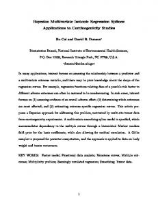
We evaluate the performance of our algorithms for regression over graphs and over V [0; T ] with the help of synthetic data. First, we present our results on more "familiar" graphs, such as lines or grids. We take advantage of what we know of these domains to test our algorithms, by adding noise to our observations and using a small fraction of our eigenvectors. Then, we present results on randomly generated small world graphs. Finally, we present two examples of the product space algorithm: one over a toy graph and the second over a larger randomly generated small world graph. For each example, results of 10 experiments are averaged. Familiar Graphs: We choose a line graph that corresponds to a uniform discretization of an interval with 500 nodes. We evaluate the results approxi) imating two functions: f1 (xi ) = sin(20 xi ) in [0; 1], and f2 (xi ) = sin(x in xi [ 20; 20]: We choose m = 2 as a good balance between smoothness and …t, and remove observations uniformly (100 nodes are not observed). Finally, we add noise " N (0; 2 ) on each node. We then choose a grid graph, a uniform 2 +y 2 ) grid of 30 30 nodes in [ 5; 5]2 ; and evaluate the function f3 (x; y) = sin(x x2 +y 2 : 38

We choose the same value of m; and we take out 180 observations uniformly. We again add gaussian noise on each node. We show the results, varying q; the number of eigenvectors: T able 1: M ean Square Error, b c and GCV score for the line graphs and the grid graph 2 2 j f2 = 0:01 j f3 = 0:01

2 f1 = 0:1 q MSE b c V (b c) 500 0:0918 1:1839 0:1172 100 0:0928 1:2114 0:1173 30 0:1019 0:1265 0:1184

j MSE b c V (b c) j 0:0095 16:1899 0:0109 j 0:0095 16:2423 0:0109 j 0:0097 16:8878 0:0109

j q MSE b c V (b c) j 900 0:0081 0:0042 0:0155 j 300 0:0106 0:0061 0:0157 j 100 0:0146 0:0103 0:0172

Our method reconstructs the signal when we add a reasonable amount of noise, and using less eigenvectors for our function representation increases M SE and the GCV scores only slightly, until we reach a number below which this representation is no longer possible. This con…rms our hypothesis: our method provides a sparse representation of the function, even in the harder cases (2 and 3). In Figure 1:, we can observe the behaviour of these quantities for q = 20 to q = 100: Target function f2(x), Estimate and 95% Bayesian intervals 10

1. 2

x 10

-3

Mean Square Error of Estimate (Over both observed and unobserved nodes)

1

0. 8 9. 5

MSE(q)

0. 6

0. 4

0. 2

9

0

-0. 2 8. 5 20

-0. 4 -20

-15

-10

-5

0

5

10

15

30

40

50

60

70

80

90

100

90

100

Nu m b e r o f Ei g e n v e c to rs q

20

GCV Estimate for the Smoothing Parameter c

GCV Score for the Estimated c

16

0. 0113

14 0. 0113

12 0. 0112

V(c)

c

10

8

0. 0112

6 0. 0111

4 0. 011

2

0 20

30

40

50

60

70

80

90

100

0. 011 20

30

40

50

60

70

80

Nu m b e r o f Ei g e n v e c to rs q

Nu m b e r o f Ei g e n v e c to rs q

Figure 1: a) Estim ate for f2 (x) b),c) and d) M SE,c and V(c) for q=20 to q=100

Small World Graph (Strogratz-Watts): We have tested on several functions over a random small world graph generated by the Watts-Strogratz generator of the Networkx Python 2:4 package. It is constructed by joining each node in a circle with its closest 2b neighbors, and rewiring each edge with probability p: We generated a graph of 1000 nodes with b = 4 and p = 0:2, and constructed three functions based on linear combinations of 4; 100 and 1000 eigenvectors. We now remove observations by sorting them according to their degree and then taking a uniform sample. Although we expected these graphs to be ’harder’on our methods because of their high local connectivity, we were glad to …nd that in the …rst two cases, the method behaves in a similar fashion to the familiar graph cases. As expected, the case with 1000 eigenvectors fails, since this function is equivalent to noise. 39

Regression on V [0; 1] : We take two graphs, sampling the interval on each case on a uniform mesh of 20 points. We model a function of the same form: f (ti ; vj ) = sin(2 xi ) log(1 + 1 (vj )), where 1 is the …rst eigenvector of the laplacian of each graph. On the …rst example, a toy graph of 4 nodes is used (we observe 3): On the second, a small world graph with 100 nodes, b = 2, p = 0:2 is used, removing 10 observations as in the small world example. We show the results in the toy graph in Figure 2: and results from low and high degree nodes from our second example: 0.8

0.2

0.2

0

0

-0 .2

-0 .2

0.02 0 -0. 02 -0. 04

-0 .6 0

0.2

0.4

0.6

0.8

1

1.5

-0 .8

0.06 0.04

-0 .4

-0 .4 -0 .6

V2 ( O b s e r v e d )

0.4

0.4

Small World Graph Product: Estimate for a LowDegree Node (Degree 1)

0.08

0.6

V1 ( O b s e r v e d )

0.6

-0. 06

0

0.2

0.4

0.6

0.8

1

0.5

V3 ( U n o b s e r v e d )

V4 ( O b s e r v e d )

-0. 08

0

0.1

0.2

0.2

0.3

0.4

0.5

0.6

0.7

0.8

0.9

1

0.9

1

Small World Graph Product: Estimate for a High Degree Node (Degree 5)

0.15

1

0.1

0.5 0.05

0

0

0

-0. 05

-0 .5 -0. 1

-1

0

0.2

0.4

0.6

0.8

1

-0 .5

0

0.2

0.4

0.6

0.8

1

-0. 15 -0. 2

Figure 2: Estim ates in our toy graph

0

0.1

0.2

0.3

0.4

0.5

0.6

0.7

We can conclude that our method provides reasonable estimates for these graphs, even for nodes where our function is not observed at all. By studying di¤erent kinds of nodes in the small world graph, we found that the only signi…cant di¤erence is that bayesian intervals tend to be wider on unobserved nodes, especially those of low degree. This follows our intuition: low degree nodes have less ’information’from other nodes to reconstruct the signal.

Acknowledgements This work was supported by NSF award IIS-0705681. We thank Kiri Wagsta¤ and the members of the UNM Machine Learning Lab for valuable discussions.

References [ABB06]

S. Agarwal, K. Branson, and S. Belongie. Higher order learning in graphs. Proceedings of the 23rd International Conference on Machine Learning ICML pages 17–24 (2006).

[BCMS04] James C. Bremer, Ronald Coifman, Mauro Maggioni, and Arthur Szlam. Di¤usion wavelet packets. (2004). [BLS00]

Türker Biyikoglu, Josef Leydold, and Peter Stadler. “Laplacian Eigenvectors of Graphs: Perron-Frobenius and FaberKrahn Type Theorems”. Lecture Notes in Mathematics. Springer Verlag (2000). 40

0.8

Figure 3: Estim ates in Sm all World Graph

[BLWY86] Bates, Lindstrom, Wahba, and Yandell. GCVPACK - routines for generalized cross validation. Technical Report 775, Univeristy of Wisconsin-Madison (1986). [BTA04]

Alain Berlinet and Christine Thomas-Agnan. “Reproducing Kernel Hilbert Spaces in Probability and Statistics”. Kluwer Academic Publishers (2004).

[Chu97]

Fan R. K. Chung. “Spectral Graph Theory”. Conference Board of the Mathematical Sciences. AMS (1997).

[CW79]

Peter Craven and Grace Wahba. Smoothing noisy data with spline functions. Springer Verlag Numerische Mathematik 31, 377– 403 (1979).

[FJP02]

Joel Friedman and Tillich Jean-Pierre. Wave equations for graphs and the edge-based laplacian. (2002).

[FT08]

Joel Friedman and Jean-Pierre Tillich. Calculus on graphs. (2008).

[GHW79] Golub, Heath, and G. Wahba. Generalized cross validation as a method for choosing a good ridge parameter. Technometrics 21(2) (May 1979). [Gu02]

Chong Gu. “Smoothing Splines ANOVA Models”. Springer Verlag (2002).

[GW93]

Chong Gu and Grace Wahba. Smoothing spline ANOVA with component-wise bayesian “con…dence intervals”. Journal of Computational and Graphical Statistics (1993).

[Iri04]

Rafael Irizarry. Choosing smoothing parameters for smoothing splines by minimizing an estimate of risk. Technical Report Working Paper 30, Johns Hopkins University, Dept. of Biostatistics (2004).

[Mah05]

Sridhar Mahadevan. (2005).

[MM07]

Sridhar Mahadevan and Mauro Maggioni. Proto-value functions: A laplacian framework for learning representation and control in markov decision processes. J. Machine Learning Research 8, 2169–2231 (2007).

[Nyc88]

Douglas Nychka. Bayesian con…dence intervals for smoothing splines. Journal of the American Statistical Association 83(404), 1134 –1143 (Dec 1988).

[RS05]

James Ramsay and B.W. Silverman. “Functional Data Analysis”. Springer Series in Statistics. Springer Verlag (2005).

Representation policy iteration.

41

UAI

[SBRZ08] Curtis Storlie, H. D. Bondell, B. J. Reich, and H. H. Zhang. The adaptive COSSO for nonparametric surface estimation and model selection. Annals of Statistics (2008). in review. [Wah90]

Grace Wahba. “Spline Models for Observational Data”. CBMSNSF Regional Conference Series in Applied Mathematics. SCIAM (1990).

[Wah03]

Grace Wahba. An introduction to (smoothing spline) ANOVA models in RKHS, with examples in geographical data, medicine, atmospheric science and machine learning. Proceedings of the 13th IFAC Symposium on System Identi…cation, Rotterdam pages 549– 559 (2003).

[ZS04]

Dengyong Zhou and Berhnard Schölkopf. A regularization framework for learning from graph data. Workshop on Statistical Relational Learning at ICML, Ban¤ , Canada (2004).

.

42