2003 Conference on Information Sciences and Systems, The Johns Hopkins University, March 12–14, 2003
Using Linear Programming to Decode Linear Codes Jon Feldman
Martin Wainwright
David R. Karger1
Laboratory for Computer Science Electrical Engineering and CS Laboratory for Computer Science MIT, Cambridge, MA, 02139 UC Berkeley, Berkeley, CA, 94720 MIT, Cambridge, MA, 02139 email: email: email:
[email protected] [email protected] [email protected] Abstract — Given a linear code and observations from a noisy channel, the decoding problem is to determine the most likely (ML) codeword. We describe a method for approximate ML decoding of an arbitrary binary linear code, based on a linear programming (LP) relaxation that is defined by a factor graph or parity check representation of the code. The resulting LP decoder, which generalizes our previous work on turbo-like codes [FK02, FWK02], has the ML certificate property: it either outputs the ML codeword with a guarantee of correctness, or acknowledges an error. We provide a precise characterization of when the LP decoder succeeds, based on the cost of pseudocodewords associated with the factor graph. We introduce the notion of the fractional distance δ of a code, defined with respect to a particular LP relaxation, and prove that the LP decoder will correct up to [δ/2] − 1 errors. For the BEC, we prove that the performance of LP decoding is equivalent to standard iterative decoding.
I. Introduction The families of turbo codes [BGT93] and low-density parity-check (LDPC) codes [Gal62] have received a lot of attention recently due to their demonstrated robustness against extremely high levels of noise. Much is understood about code design and error-correcting performance within these families (for a survey, see [Mac03]). Despite this attention, however, the current understanding of finite-length turbo codes and LDPC codes is still limited. For instance, the conditions under which the conventional belief-propagation (BP) decoders [MDC98] succeed, or even converge, are not fully understood, nor are there satisfying analytical bounds explaining their superb performance observed in practice. Decoding via Linear Programming. In previous work [FK02, FWK02], we introduced the approach of decoding any “turbo-like” code based on network flow and linear programming relaxation techniques. We gave a precise combinatorial characterization of the conditions under which this decoder succeeds. We used properties of this LP decoder to design a rate-1/2 Repeat-Accumulate (RA) code (a certain class of simple turbo codes), and proved an upper bound on the probability of decoding error. We also showed how to derive a more classical iterative algorithm whose performance is identical to that of our LP decoder.
Our Contribution. In this paper, we generalize our methods to an arbitrary binary linear code. We define the linear code linear program (LCLP), which is an approximation to the maximum-likelihood (ML) decoding problem based on the method of linear programming (LP) relaxation. An LP decoder is a decoder based on the LCLP relaxation. Experiments show that the performance of LP decoding is on par with the iterative min-sum algorithm. In addition, as in turbo-like codes, the LP decoder has the ML certificate property; whenever it outputs a codeword, it is guaranteed to be the ML codeword. None of the standard iterative methods are known to have this desirable property. We give an exact combinatorial characterization of the conditions for LP decoding success. We use the channel model to define a cost function on the bits such that the lowest cost codeword is the ML codeword. We define the set of pseudocodewords, which is a superset of the set of codewords, and we prove that the LP decoder always finds the lowest cost pseudocodeword. Thus, the LP decoder succeeds if and only if the lowest cost pseudocodeword is actually the transmitted codeword. Our notion of a pseudocodeword unifies other known results for particular cases of codes and channels. For tail-biting trellises, the pseudocodewords analyzed in this paper are equivalent to those introduced by Forney et al. [FKKR01]. For the case of the binary erasure channel (BEC), pseudocodewords are exactly stopping sets, as defined by Di et al. [DPR+ 02]. Thus, the performance of the LP decoder is equivalent to iterative methods in both these cases. Also, when applied to the analysis of computation trees for min-sum decoding, pseudocodewords have a connection to the deviation sets defined by Wiberg [Wib96]. We define the notion of the fractional distance δ of a linear code, which is a generalization of the classical distance. In analogy to the performance guarantees of exact ML decoding with respect to classical distance, we prove that the LP decoder can correct up to δ/2 − 1 errors in the binary symmetric channel (BSC). We prove that the fractional distance of a linear code with check degree at least three is at least exponential in the girth of the graph associated with that code. Thus, given a graph with logarithmic girth, the fractional distance can be lower bounded by Ω(n1−ǫ ), for some constant ǫ, where n is the code length. For the case of LDPC codes, we show how to compute the fractional distance efficiently. This fractional distance is not only useful for evaluating the performance of the code under LP decoding, but it also serves as a lower bound on the true distance of the code.
II. Background 1 Research supported by NSF contract CCR-9624239 and a David and Lucille Packard Foundation Fellowship.
A linear code C with parity check matrix A can represented by a Tanner or factor graph G, which is defined in the following
way. Let I = {1, . . . , n} and J = {1, . . . , m} be indices for the columns (respectively rows) of the n × m parity check matrix of the code. With this notation, G is a bipartite graph with independent node sets V = {vi | i ∈ I} and C = {cj | j ∈ J }. We refer to the nodes in V as variable nodes, and the nodes in C as check nodes. All edges in G have one endpoint in V and the other in C. For each i, j, the edge (vi , cj ) is included in G if and only if Aij = 1. The neighborhood of a check node cj , denoted by N (cj ), is the set of variable nodes vi that are incident to cj in G. Similarly, we let N (vj ) represent the set of check nodes incident to a particular variable node vj in G. We will often use N (j) to denote the set of indices i such that vi ∈ N (cj ); similarly, N (i) denotes the set of indices j for which cj ∈ N (vi ). The particular meaning should be clear from the context; generally, we will use i to denote variable nodes (code bits), and j to denote parity checks. Imagine assigning to each variable node vi a value in {0, 1}, representing the value of a particular code bit. A parity check node cj is “satisfied” if the collection of bits assigned to the variable nodes in its neighborhood N (cj ) have even parity. The binary vector v = (v1 , . . . , vn ) is codeword if and only if all check nodes are satisfied. Figure 1 shows an example of a linear code and its associated Tanner graph. In this Hamming code, if we set v1 = v3 = v4 = v7 = 1, and v2 = v5 = v6 = 0, then the neighborhood of every check node has even parity. Therefore, this represents a codeword, which we can write as 1011001. Other codewords include 1111111, 0101001, and 1010110.
v2
v1
v3
c1
c2 v4
v5
v6 c3 v7
Figure 1. A factor graph for the (7,4,3) Hamming Code. The nodes {vi } drawn in open circles correspond to variable nodes, whereas nodes {cj } in black squares correspond to check nodes.
III. Decoding with Linear Programming In this section, we formulate the ML decoding problem for an arbitrary binary linear code, and show that it is equivalent to solving a linear program over the codeword polytope. We then define a modified linear program that represents a relaxation of the exact problem. Due to space limitations, we leave out most of the proofs in this paper, and defer them to the full version. A. Exact ML decoding A codeword y is sent over a noisy channel, and a corrupted word yˆ is received. Given the received word yˆ, the ML decoding problem is find the codeword that maximizes the likelihood (or, equivalently minimizes the negative log likelihood) of observing yˆ under P the channel model. This cost function can be written as n ˆi ]/Pr[0 | yˆi ]) is i=1 γi vi , where γi = − log(Pr[1 | y the negative log likelihood ratio (LLR) at each variable node. For example, given a binary symmetric channel (BSC) with crossover probability p, we set γi = − log[(1 − p)/p] if the received bit yˆi = 1, and γi = − log[p/(1 − p)] if yˆi = 0. The
interpretation of γi is the “cost” of decoding vi = 1. We will frequently exploit the fact that the cost vector γ can be uniformly rescaled without affecting the solution of the ML problem. In the BSC, for example, rescaling by − log[p/(1 − p)] allows us to assume that γi = −1 if yˆi = 1, and γi = +1 if yˆi = 0. To motivate our linear programming (LP) relaxation, we first show how ML decoding can formulated as an equivalent LP. For a given code C, we define the codeword polytope to be the convex hull of all possible codewords: ( ) X X CH(C) = λv v : λv > 0, λv = 1 v∈C
v∈C
Every point in CH(C) corresponds to a vector f = (f1 ,P . . . , fn ), where element fi is defined by the summation fi = v λv vi . We Pn can define ML decoding as the problem of minimizing i=1 γi fi subject to the constraint f ∈ CH(C). This formulation is a linear program, since it involves minimizing a linear cost function over the polytope CH(C). The vertices of a polytope are those points that cannot be expressed as convex combinations of other points in the polytope. A key fact is any linear program attains its optimum at a vertex of the polytope. Consequently, the optimum will always be attained at a vertex of CH(C), and these vertices are in one-to-one correspondence with codewords. B. Linear programming relaxation In this LP formulation of exact ML decoding, the complexity of the problem lies in the nature of the codeword polytope. Although CH(C) can be characterized by a finite number of linear constraints, the number of constraints is exponential in the code length n. Therefore, our strategy will be to formulate a relaxed polytope, one that contains all the codewords, but has a more manageable representation. More concretely, we motivate our LP relaxation with the following observation: each check node in a factor graph defines a local code, and the global code corresponds to the intersection of all the local codes. In LP terminology, each check node defines a local codeword polytope (the set of convex combinations of local codes), and our global polytope is the intersection of all of these polytopes. To define a local codeword polytope, we consider the set of variable nodes {vi | i ∈ N (j)} that are neighbors of a given check node cj . Of interest are subsets S ⊆ N (j) that index an even number of variable nodes, since each such subset corresponds to a local codeword, defined by setting variable node vi = 1 for each index i ∈ S, and vi = 0 for each i ∈ / S. For each S in the set Ej = {S ⊆ N (j) : |S| even}, we introduce an auxiliary LP variable wj,S , which is an indicator for the local codeword associated with S. Note that the variable wj,∅ is also present for each parity check, and it represents setting all variables in N (j) equal to zero. As indicator variables, the variables {wj,S } must satisfy the constraints: ∀j ∈ J , S ∈ Ej ,
0 6 wj,S 6 1.
(1)
Moreover, since each parity check can only be “satisfied” with one particular even-sized subset of nodes in its neighborhood set to one, we must have: X ∀j ∈ J , wj,S = 1. (2) S∈Ej
Finally, the indicator fi at each variable node vi must belong to the local codeword polytope associated with cj (for each j ∈ N (i)). This leads to the constraint: X ∀ (i, j) ∈ I × J , fi = wj,S . (3) S∈Ej S∋vi
Let the polytope P be the set of points (f, w) such that equations (1) , (2), and (3) hold. Overall, the LCLP relaxation corresponds to the problem: minimize
n X
γi fi s.t. (f, w) ∈ P
(4)
i=1
An integral solution to a linear program is a feasible point whose values are all integers. We begin by observing that there is a one-to-one correspondence between codewords and integral solutions (f, w) to LCLP: Lemma 1 For all integral solutions (f, w) to LCLP, the sequence (f1 , . . . , fn ) represents a codeword. Furthermore, for all codewords (v1 , . . . , vn ), there is a setting of the variables w such that (f, w) is an integral solution, where f = v. One consequence of this claim is that any integral optimal solution to LCLP specifies the ML codeword. Given a cyclefree factor graph, it can be shown that any optimal solution to LCLP is integral, so that LCLP is an exact formulation of the ML decoding problem. In contrast, for a factor graph with cycles, the optimal solution to LCLP may not be integral. Take, for example, the Hamming code in Figure 1. Suppose that we define a cost vector γ as follows: for variable node v1 , set γ1 = −7/4, and for all other nodes vi , set γi = +1. It is not hard to verify that under this cost function, all codewords have non-negative cost: any codeword with negative cost would have to set v1 = 1, and therefore set at least two other vi = 1, for a total cost of at least +1/4. Consider, however, the following fractional solution to LCLP: first, set f = [1, 1/2, 0, 1/2, 0, 0, 1/2] and then for check node 1, set w1,{v1 ,v2 } = w1,{v1 ,v4 } = 1/2; at check node 2, assign w2,{v2 ,v4 } = w2,∅ = 1/2; and lastly at check node 3, set w3,{v4 ,v7 } = w3,∅ = 1/2. It can be verified that (f, w) satisfies all of the LCLP constraints. However, the cost of this solution is −1/4, which is strictly less than the cost of any codeword. The analysis to follow will provide further insight into the nature of such fractional (i.e., non-integral) solutions to LCLP. We note that the local codeword constraints (3) are analogous to those enforced in the Bethe formulation of belief propagation [YFW02].
codeword), but the ML codeword is not what was transmitted. In this latter case, the code itself has failed, so that even exact ML decoding would make an error. We use the notation Pr[err | y] to denote the probability that the LP decoder makes an error, given that y was transmitted. By Lemma 1, there is some feasible solution (y, w0 ) to LCLP corresponding to the transmitted codeword y. We can characterize the conditions under which LP decoding will succeed as follows: Theorem 2 Suppose the codeword y is transmitted. If all feasible solutions to LCLP other than (y, w0 ) have cost more than the cost of y, the LCLP decoder succeeds. If some solution to LCLP has cost less than the cost of y, the decoder fails. In the degenerate case where (y, w0 ) is one of multiple optima of LCLP, the decoder may or may not succeed. We will be conservative and consider this case to be decoding failure, and so by Theorem 2: " # X X Pr[err | y] = Pr ∃(f, w) ∈ P, f 6= y : γi fi 6 γi yi (5) i
i
In the analysis to follow, we provide combinatorial characterizations of decoding success, and analyze the performance of LP decoding in various settings. A. The All-Zeros Assumption When analyzing linear codes, it is common to assume that the codeword sent over the channel is the all-zeros vector (i.e., y = 0n ), since it tends to simplify analysis. In the context of our LP relaxation, however, the validity of this assumption is not immediately clear. In this section, we prove that one can make the all-zeros assumption when analyzing LCLP. Specifically, we show that for all codewords y, Pr[err | y] = Pr[err | 0n ]. In the BSC, let E be the set of bits flipped by the channel; i.e., E = {i : yˆi 6= yi }. For all i ∈ I, let γi0 = −1 if bit i ∈ E, and γi0 = +1 otherwise. Note that if the all-zeros word was transmitted, then γ 0 would represent the cost function. The following lemma establishes a one-to-one correspondence between the points of P under cost function γ, and the points of P under cost function γ 0 : Lemma 3 Fix some codeword y. For every (f, w) ∈ P , r r f 6= y, there ∈ P , f r 6= 0n , such that P(f 0, wr ) P P is some P 0 n i γi 0i . Furthermore, for i γi fi − i γi yi = i γi fi − r r r n every (f ,P w ) ∈ P , fP6= 0 , there (f, w) ∈ P , f 6= y, P is some P such that i γi0 fir − i γi0 0n i = i γi fi − i γi yi . This lemma, along with equation (5), gives: " # X 0 r X 0 n r r r n Pr[err|y] = Pr ∃(f , w ) ∈ P, f 6= 0 : γi fi 6 γi 0i i
IV. Analysis of LP decoding Overall, the decoding algorithm based on LCLP consists of the following steps. We first solve the LP in equation (4) to obtain (f ∗ , w∗ ). If f ∗ is integral (all zeros and ones), we output it as the optimal codeword; otherwise, f ∗ is fractional, and we output an “error.” Lemma 1 implies that this algorithm has the ML certificate property: if the algorithm outputs a codeword, it is guaranteed to be the ML codeword. When using the LP decoding method, an error can arise in one of two ways. Either the LP optimum f ∗ is not integral, in which case the algorithm outputs “error”; or, the LP optimum may be integral (and therefore correspond to the ML
i
= Pr[err | 0n ].
A similar result can be shown for the AWGN channel. From this point forward in our analysis of LP decoding, we assume that the all-zeros codeword was the transmitted codeword, and so γ = γ 0 . Since the all-zeros codeword has zero cost, Theorem 2 says that the LP decoder will fail only if there is some non-zero point in P with cost less than or equal to zero. B. Decoding Efficiency The linear program can be solved with any generic LP solver, such as the simplex algorithm [Sch87], which is often efficient in practice, or the Ellipsoid algorithm [GLS81],
which has better worst-case guarantees. To establish that the LP solver will run efficiently using one of these two methods, we must show that the LP either has a limited number of variables and constraints, or a separation oracle. Let dr denote the maximum check (right) degree of the code. As stated, LCLP has O(n + m2dr ) variables and constraints. For turbo and LDPC codes, this complexity is linear in n, since dr is constant. For arbitrary linear codes, we use results of Yannakakis [Yan91] to obtain a characterization of LCLP with O(n + mdr2 ) = O(n3 ) variables and constraints. We leave these details for the complete version of the paper.
V. Fractional Distance A classical quantity associated with a code is its distance, which for a linear code is equal to the minimum weight of any non-zero codeword. In this section, we introduce a fractional analog of distance, and use it to prove additional results on the performance of LP decoding. Roughly speaking, the fractional distance is the minimum weight of any non-zero LCLP optimum; since all codewords are potential optima, the fractional distance is a lower bound on the true distance. A. Definitions and Basic Properties P Define the weight of a point (f, w) in the polytope P as i fi . Let VP denote the set of vertices of the polytope P , and define VP− = VP \ (f 0 , w0 ) to be the set of all vertices excluding that corresponding to the all-zeros codeword. Since there is a one-to-one correspondence between codewords and integral vertices of P , the distance of the code is equal to the minimum weight of an integral vertex in VP− . However, the relaxed polytope P may have additional non-integral vertices, as illustrated, in particular, by our earlier example with the Hamming code. Since the optimal solution to LCLP will always be a vertex of P , it is natural to define the minimum weight of any vertex in VP− as an analog to the distance. It turns out that we can obtain a slightly sharper definition by exploiting the fact that not all vertices of P can be optimal solutions to instances of LCLP. Let Q be the projection of P onto the subspace defined defined by the variables f1 , . . . , fn . More formally, this projection is defined as Q = {f : ∃w s.t. (f, w) ∈ P }. As stated previously, any optimal solution (f ∗ , w∗ ) to LCLP must be a vertex of P . However, the fact that the cost function for LCLP only affects the variables f1 , . . . , fn implies that f ∗ must also be a vertex of the projection Q. (In general, not all vertices of P will be projected to vertices P of Q.) For a− point f in Q, be the set of define the weight of f to be i fi , and let VQ non-zero vertices of Q. With this notation, we define the fractional distance of a − code to be the minimum weight of any vertex in VQ . Note that this fractional distance is always a lower bound on the classical distance of the code, since every codeword is contained in − VQ . Moreover, the performance of LP decoding is tied to this fractional distance, as we make precise in the following: Theorem 4 For a code G with fractional distance δ, the LP decoder is successful if fewer than δ/2 bits are flipped by the binary symmetric channel. Proof: Suppose the LP decoder fails; i.e., the optimal solution (f ∗ , w∗ ) to LCLP has f ∗ 6= 0n . We know that f ∗ must be a − vertex of Q. Since f ∗ 6= 0n , f ∗ ∈ VQ . This implies that P ∗ i fi > δ, since the fractional distance is at least δ.
Recall that E = {i : yˆi 6= yi } is the set of bits flipped by the channel. We can write the cost of f ∗ as the following: X i
γi fi∗ =
X i∈E /
fi∗ −
X
fi∗ .
(6)
i∈E
Since fewer than δ/2 bits are P flipped by the channel, we ∗ have P that |E| < δ/2, and so It follows i∈E fi < δ/2. P ∗ ∗ that f > δ/2, since f > δ. Therefore, by (6), i i i∈E / i P ∗ i γi fi > 0. However, by Theorem 2 and the fact that the decoder failed, the optimal solution (f ∗ ,P w∗ ) to LCLP must have cost less than or equal to zero; i.e., i γi fi 6 0. This is a contradiction. Note again the analogy to the classical case: just as exact ML decoding has a performance guarantee in terms of classical distance, Theorem 4 establishes that the LP decoder has a performance guarantee specified by the fractional distance of the code. B. Lower Bound on the Fractional Distance The following theorem asserts that the fractional distance is exponential in the girth of G. It is analogous to an earlier result of Tanner [Tan81], which provides a similar bound on the classical distance of a code in terms of the girth of the associated Tanner graph. Theorem 5 Let G be a Tanner graph with variable degree dℓ > 3 and check degree dr > 2, and let g be the girth of G. Then the fractional distance is at least (2/dr )(dℓ − 1)g/4−1 . One consequence of Theorem 5 is that the fractional distance is at least Ω(n1−ǫ ) for some constant ǫ, for any graph G with girth Ω(log n). Note that there are many known constructions of such graphs [e.g., RV00]. Although Theorem 5 does not yield a bound on the WER for the BSC, it demonstrates that LP decoding can correct Ω(n1−ǫ ) errors for any code defined by a graph with logarithmic girth. Moreover, with an alternative definition of fractional distance, we can provide a somewhat sharper statement, showing in particular that LP decoding can correct up to (1/2)(dℓ − 1)g/4−1 errors in the channel. C. Computing the Fractional Distance In contrast to the classical distance, the fractional distance of an LDPC code can be computed efficiently. Since the fractional distance is a lower bound on the real distance, we thus have an efficient algorithm to give a non-trivial lower bound the distance of an LDPC code. To compute the fractional distance, we must compute the − minimum weight vertex in VQ . We first consider a more general problem: given the m facets of a polytope R over vertices (x1 , . . . , xn ), a specified vertex x0 of R, and a linear function ℓ(x), find the vertex in R other than x0 that minimizes ℓ(x). An efficient algorithm for this problem is the following: let F be the set of all facets of R on which x0 does not sit. Now for each facet in F , intersect R with the facet to obtain R′ , and then optimize ℓ(x) over R′ . The minimum value obtained over all facets in F is the minimum of ℓ(x) over all vertices other than x0 . The running time of this algorithm is proportional to |F | < m calls to an LP solver. For our problem, we are interested in the polytope Q, and the special vertex 0n ∈ Q. In order to run the above procedure, we must provide a small representation of Q = {f : ∃w s.t. (f, w) ∈ P }. The following definition of Q in
terms of constraints on f was derived from the parity polytope of Yannakakis [Yan91]. We first enforce 0 6 fi 6 1 for all i ∈ I, and then for all j ∈ J , T ⊆ N (j), |T | odd, we require: X X fi + (1 − fi ) 6 |N (j)| − 1. (7) i∈T
node vi , and uj,S copies of each check node cj , with “label” S. We refer to the copies of the variable node as (vi1 , . . . , vihi ). The edges of the graph are connected according to member-
v11
i∈(N (j)\T )
c1
v21 c2
Thus, the number of facets in Q has an exponential dependence on the check degree of the code. For an LDPC code, the number of facets will be linear in n, so that we can compute the exact fractional distance efficiently. For arbitrary linear codes, we can still compute the minimum weight non-zero vertex of P , which provides a lower bound on the fractional distance, and hence a (possibly weaker) lower bound on the classical distance.
Figure 2. The graph of a pseudocodeword for the (7,4,3)
VI. Pseudocodewords
Hamming code. In this particular pseudocodeword, there are two copies of node v1 , and also two copies of check c1 .
In this section, we introduce the concept of a pseudocodeword, which we will define as a scaled version of a solution to LCLP. As a consequence, Theorem 2 will hold for pseudocodewords in the same way that it holds for solutions to LCLP. The following definition of a codeword motivates the notion of a pseudocodeword. Let h be a vector in {0, 1}n , and let u be a setting of non-negative integer weights, one weight uj,S for each check j and S ∈ (Ej \ {∅}). We say that (h, u) is a codeword P if, for all edges (vi , cj ) in the Tanner graph G, hi = S∈Ej ,S∋i uj,S . This corresponds exactly to the consistency constraint (3) in LCLP. It is not difficult to see that this construction guarantees that the binary vector h is always a codeword of the original code. We obtain the definition of a pseudocodeword (h, u) is by removing the restriction hi ∈ {0, 1}, and instead allowing each hi to take on arbitrary non-negative integer values. With this definition, any codeword is (trivially) a pseudocodeword as well; moreover, any sum of codewords is a pseudocodeword. However, in general there exist pseudocodewords that cannot be decomposed into a sum of codewords. As an illustration, consider the Hamming code of Figure 1; earlier, we constructed a fractional LCLP solution for this code. If we simply scale this fractional solution by a factor of two, the result is a pseudocodeword (h, u) of the following form. We begin by setting h = [2, 1, 0, 1, 0, 0, 1]. To satisfy the constraints of a pseudocodeword, set u1,{v1 ,v2 } = u1,{v1 ,v4 } = u2,{v2 ,v4 } = u2,∅ = u3,{v4 ,v7 } = u3,∅ = 1. This pseudocodeword cannot be expressed as the sum of individual codewords. Using simple scaling arguments, and the all-zeros assumption, we can restate Theorem 2 in terms of pseudocodewords as follows: Theorem 6 If all non-zero pseudocodewords have positive cost, the LCLP decoder succeeds. If some non-zero pseudocodeword has negative cost, the LCLP decoder fails. A. Pseudocodeword Graphs Pseudocodewords have a graphical representation that is often helpful. We begin by observing any codeword corresponds to a particular subgraph of the Tanner graph G. In particular, the vertex set of this subgraph consists of all the variable nodes for which vi = 1, as well as all check nodes to which these variable nodes are incident. Any pseudocodeword (h, u) can be associated with a graph H in an analogous way. The vertex set of the graph H consists of hi copies of each
v12
c1
v41 c3 v71
ship in the sets S. More precisely, consider an edge (vi , cj ) in G. There are hi copies of vi in H, and there are also hi copies of cj labeled with sets S that include i. Connect these node sets using an arbitrary one-to-one correspondence. Figure 2 gives the graph of the pseudocodeword example given earlier. After all connections in H are made in this manner, every check node in H will be connected to an even number of variable nodes (none of them being copies of one another), and every variable node corresponding to vi will be connected to exactly one copy of each check node cj in N (vi ). The cost of this graph is the sum of the costs γi of the variable nodes in the graph, and is clearly equal to the cost of the pseudocodeword from which it was derived. This graphical representation of a pseudocodeword is helpful in making connections with other notions of pseudocodewords in the literature. For example, the deviation sets defined by Wiberg [Wib96] can be compared to pseudocodeword graphs. On tail-biting trellises, pseudocodeword graphs correspond to those analyzed by Forney et al. [FKKR01]. In the next section, we will use these graphs to show that on the BEC, pseudocodewords are exactly stopping sets. B. Stopping sets in the BEC In the binary erasure channel (BEC), bits are not flipped but rather erased. Consequently, for each bit, the decoder receives either 0, 1, or an erasure. If either symbol 0 or 1 is received, then it must be correct. On the other hand, if an erasure (which we denote by x) is received, there is no information about that bit. It is well-known [DPR+ 02] that in the BEC, the iterative belief propagation (BP) decoder fails if and only if a so-called stopping set exists among the erased bits. The main result of this section is that stopping sets are the special case of pseudocodewords on the BEC, and so LP decoding exhibits the same property. We can model the BEC in LCLP with our cost function γ. As in the BSC, γi = −1 if the received bit yˆi = 1, and γi = +1 if yˆi = 0. If yˆi = x, we set γi = 0, since we have no information about that bit. Note that under the all-zeros assumption, all the costs are non-negative, since no bits are flipped. Therefore, Theorem 6 implies that either the LP decoder will succeed, or there will be a non-zero pseudocodeword with zero cost. Let E be the set of code bits erased by the channel. A subset S ⊆ E is a stopping set if all the checks in the neighborhood ∪i∈S N (i) of S have degree at least two with respect to S.
Theorem 7 Under the BEC, there is a non-zero pseudocodeword with zero cost if and only if there is a stopping set. Therefore, the performance of LP and BP decoding are equivalent for the BEC. In the statement, we have assumed that both the iterative and the LCLP decoders fail when the answer is ambiguous. For the iterative algorithm, this ambiguity corresponds to the existence of a stopping set; for the LCLP algorithm, it corresponds to a non-zero pseudocodeword with zero-cost, and hence multiple optima for the LP.
VII. Tighter relaxations It is important to observe that LCLP has been defined with respect to a specific factor graph. Since a given code has many such representations, there are many possible LPbased relaxations, and some may be better than others. Of particular significance is the fact that adding redundant parity checks to the factor graph, though not affecting the code, provides new constraints for the LP relaxation, and will in general strengthen it. For example, returning to the (7, 4, 3) Hamming code of Figure 1, suppose we add a new check node whose neighborhood is {v1 , v3 , v5 , v6 }. This parity check is redundant for the code, since it is simply the mod two sum of c1 and c2 . However, the linear constraints added by this check tighten the relaxation; in fact, they render the pseudocodeword f = [1, 1/2, 0, 1/2, 0, 0, 1/2] infeasible. Whereas redundant constraints may degrade the performance of BP decoding (due to the creation of small cycles), adding new constraints can only improve LP performance. In addition to redundant parity checks, there are various generic ways in which an LP relaxation can be strengthened [e.g., LS91, SA90]. Such “lifting” techniques provide nested sequence of relaxations increasing in both tightness and complexity, the last of which is exact (albeit with exponential complexity). It would be interesting to analyze how quickly such a sequence of relaxations approaches CH(C). Finally, the fractional distance of a code, as defined here, is also a function of the factor graph representation of the code. Fractional distance yields a lower bound on the true distance, and the quality of this bound could also be improved by adding redundant constraints, or other methods of tightening the LP.
VIII. Discussion We have described an LP-based decoding method, and proved a number of results on its error-correcting performance. Central to this characterization is the notion of a pseudocodeword, which corresponds to a rescaled solution of the LP relaxation. Our definition of pseudocodeword unifies previous work on iterative decoding [e.g., FKKR01, Wib96, DPR+ 02]. We also introduced the fractional distance of a code, a quantity which shares important properties with the classical notion. We proved a guarantee on the error-correcting performance of LP decoding in terms of the fractional distance that parallels the well-known link between exact ML decoding and the classical distance. There are a number of open questions and future directions suggested by the work presented in this paper. It is likely that the fractional distance bound in this paper can be substantially strengthened by consideration of graph-theoretic properties other than the girth (e.g., expansion), or by looking at random codes. A linear lower bound on the fractional distance would yield a decoding algorithm with exponentially small error rate.
In previous work on RA codes [FK02], we were able to prove a bound on the error rate of LP decoding stronger than that implied by the minimum distance. It would be interesting to see the same result in the more general setting of LDPC codes or linear codes. Perhaps an analysis similar to that of Di et al. [DPR+ 02], which was performed on stopping sets in the BEC, could be applied to pseudocodewords in other channel models.
References [BGT93] C. Berrou, A. Glavieux, and P. Thitimajshima. Near Shannon limit error-correcting coding and decoding: turbocodes. Proc. IEEE International Conference on Communication (ICC), Geneva, Switzerland, pages 1064–1070, May 1993. [DPR+ 02] C. Di, D. Proietti, T. Richardson, E. Telatar, and R. Urbanke. Finite length analysis of low-density parity check codes. IEEE Trans. Info Theory., 48(6), 2002. [FK02] Jon Feldman and David R. Karger. Decoding turbo-like codes via linear programming. Proc. 43rd annual IEEE Symposium on Foundations of Computer Science (FOCS), November 2002. [FKKR01] G.D. Forney, Jr., R. Koetter, F. R. Kschischang, and A. Reznick. On the effective weights of pseudocodewords for codes defined on graphs with cycles. In Codes, systems and graphical models, pages 101–112. Springer, 2001. [FWK02] Jon Feldman, Martin J. Wainwright, and David R. Karger. Linear programming-based decoding of turbo-like codes and its relation to iterative approaches. In Proc. Allerton Conf. Comm., Control and Computing, October 2002. [Gal62] R. Gallager. Low-density parity-check codes. IRE Trans. Inform. Theory, IT-8:21–28, Jan. 1962. [GLS81] M. Grotschel, L. Lov´ asz, and A. Schrijver. The ellipsoid method and its consequences in combinatorial optimization. Combinatorica, 1(2):169–197, 1981. [LS91] L. Lov´ asz and A. Schrijver. Cones of matrices and setfunctions and 0-1 optimization. SIAM Journal on Optimization, 1(2):166–190, 1991. [Mac03] David MacKay. Information Theory, Inference and Learning Algorithms. Unpublished Manuscript. http://www.inference.phy.cam.ac.uk/mackay/itprnn/book.html., 2003. [MDC98] R. McEliece, D.MacKay, and J. Cheng. Turbo decoding as an instance of Pearl’s belief propagation algorithm. IEEE Journal on Selected Areas in Communications, 16(2):140–152, 1998. [RV00] Joachim Rosenthal and Pascal O. Vontobel. Constructions of LDPC codes using Ramanujan graphs and ideas from Margulis. In Proc. of the 38-th Annual Allerton Conference on Communication, Control, and Computing, pages 248–257, 2000. [SA90] H. D. Sherali and W. P. Adams. A hierarchy of relaxations between the continuous and convex hull representations for zeroone programming problems. SIAM Journal on Optimization, 3:411–430, 1990. [Sch87] A. Schrijver. Theory of Linear and Integer Programming. John Wiley, 1987. [Tan81] R. M. Tanner. A recursive approach to low complexity codes. Information Theory, IEEE Transactions on, 27(5):533– 547, 1981. [Wib96] N. Wiberg. Codes and Decoding on General Graphs. PhD thesis, Linkoping University, Sweden, 1996. [Yan91] Mihalis Yannakakis. Expressing combinatorial optimization problems by linear programs. Journal of Computer and System Sciences, 43(3):441–466, 1991. [YFW02] J. S. Yedidia, W. T. Freeman, and Y. Weiss. Understanding belief propagation and its generalizations. Technical Report TR2001-22, Mitsubishi Electric Research Labs, January 2002.