Abstract. We study the applicability of meshfree approximation schemes for the solution of multi-asset American option problems. In particular, we consider a ...
Using Meshfree Approximation for Multi-Asset American Option Problems G. E. Fasshauer∗, A. Q. M. Khaliq†and D. A. Voss‡
Abstract We study the applicability of meshfree approximation schemes for the solution of multi-asset American option problems. In particular, we consider a penalty method which allows us to remove the free and moving boundary by adding a small and continuous penalty term to the Black-Scholes equation. Time discretization is achieved by a linearly implicit θ method. A comparison with results obtained recently by two of the authors using a linearly implicit finite difference method is included.
1
Introduction
We consider the Black-Scholes model for American basket options with a nonlinear penalty source term. In the penalty approach, the free boundary is removed by adding a small continuous penalty term to the Black-Scholes equation. The problem can then be solved on a fixed domain. This kind of penalty method was introduced by Zvan et al. [25] for American options with stochastic volatility by adding a source term to the discrete equation. In [7] it was established that their penalty method applied together with a finite volume spatial discretization leads to a quadratically convergent numerical scheme. The authors of that paper also emphasize some of the advantages of penalty methods, namely the same technique applies to one-dimensional and multi-dimensional problems. Moreover, the technique can be used for any type of discretization, in any dimension, and on structured as well as unstructured meshes. It is also possible to use the penalty approach to handle American options together with other nonlinearities. A small continuous source term was added to the Black-Scholes partial differential equation by Nielsen et al. [16, 17] for both single and two-asset American options. The authors illustrated the performance of various numerical schemes based on theta methods for temporal integration and replacing the spatial derivatives (i.e., derivatives with respect to the asset prices) by finite difference approximations. The multi-asset case was also studied by two of the authors of this work [12] using centered finite differences to approximate the spatial derivatives. In this paper we consider a meshfree radial basis function (RBF) approach as spatial approximation for the numerical solution of the American options value and its ∗
Department of Applied Mathematics, Illinois Institute of Technology, Chicago, IL 60616, USA Department of Mathematics, Knox College, Galesburg, IL 61401, USA ‡ Department of Mathematics, Western Illinois University, Macomb, IL 61455, USA †
derivatives in the Black-Scholes equation. It is known that globally supported RBFs are capable of providing a highly accurate spatial approximation to the solution (for the approximation properties of RBFs in the PDE case see, e.g., [5, 8]). The RBF approach does not require the generation of a grid as in the finite difference method. Since many of the radial basis functions (such as Gaussians and generalized multiquadrics) are infinitely continuously differentiable, the higher order partial derivatives of the option value that are used in hedging can be computed directly by using the derivatives of the basis functions.
2
A Penalty Method for American Basket Options
A basket option is an option whose price is based on multiple underlying assets. We assume there are s such assets whose price at time t is denoted by S(t) = (S1 (t), . . . , Ss (t)). The value P (S, t) of the American put option can be determined by solving a multidimensional Black-Scholes equation. Since an American option permits early exercise this problem is usually formulated as a moving boundary problem (see, e.g., [20]). If we introduce the notation S(t) = (S1 (t), . . . , Ss (t)) to represent the moving boundary, T for the time of expiry, denote the volatility of the i-th underlying asset by σi , let r be the risk free interest rate (assumed to be fixed throughout the time period of interest), Di the dividend paid by asset i, and let ρij be the correlation between assets i and j, then we get the following linear parabolic partial differential equation s
s
s
X ∂P 1 XX ∂2P ∂P + + − rP = 0, ρij σi σj Si Sj (r − Di )Si ∂t 2 ∂Si Sj ∂Si i=1 j=1
(1)
i=1
Si > Si (t), i = 1, . . . , s, 0 ≤ t < T, known as the Black-Scholes equation for multi-asset problems. The payoff function of the American put is given by F (S) = max(E −
s X
αi Si , 0),
i=1
where E is the exercise price of the option and αi are given constants. If we define the domain Ω = {(S1 , . . . , Ss ) : Si > 0, i = 1, . . . , s}, then we can formulate the terminal condition for (1) as P (S, T ) = F (S),
S ∈ Ω.
(2)
Along the moving boundary we require P (S(t), t) = F (S(t)), F (S(T )) = 0.
(3) (4)
Equations (3) and (4) ensure that the exercise value and the continuation value of the option are the same along the exercise boundary. To have a smooth transition we 2
also require that the gradient of the option value (with respect to the underlying asset prices) is continuous at the boundary. This so-called smooth pasting condition is given by ∂P (S, t) = −αi , i = 1, . . . , s. (5) ∂Si More details about the conditions along the exercise boundary are given in [20]. Finally, the following boundary conditions are added: lim P (S, t) = 0,
Si →∞
S ∈ Ω, i = 1, . . . , s,
P (S, t) = gi (S, t),
S ∈ Ωi , i = 1, . . . , s.
(6) (7)
Here the Ωi denote the boundaries of Ω along which the price Si = 0. Since the BlackScholes equation assumes a lognormal distribution model for the asset price changes, it follows that if one of the asset prices is zero at time t∗ , then the asset will be worthless for any t ≥ t∗ . Thus, the functions gi specifying the boundary conditions are the solutions of associated (s − 1)-dimensional Black-Scholes problems. Moreover, for put options, the contract becomes worthless as the price of any of the underlying assets tends to infinity. Therefore, the right-hand side of (6) is zero. Since for an American option early exercise is permitted, the value of the option must satisfy the positivity constraint P (S, t) − F (S) ≥ 0,
S ∈ Ω.
(8)
Our approach to eliminating the moving boundary from the above formulation follows [12, 16, 17]. We will add a penalty term to the Black-Scholes equation (1) and thereby convert the problem to one on a fixed domain. This transformation was suggested in [25] and later refined in [17] (both for the case of single asset options, see also the references [3, 13, 23]). In [16] a penalty formulation for multi-asset options was presented, and it was proven that the approximate option prices obtained via the penalty approach satisfy a number of fundamental properties of the American option problem such as the positivity constraint (8). Thus, the penalty term is chosen so that the solution stays above the payoff function as the solution approaches expiry. Moreover, far from the barrier q (see (10) below) the penalty term is small enough so that the PDE still resembles the Black-Scholes equations very closely. It is easily seen that a penalty term of the form �C (9) P� + � − q satisfies these requirements. Here 0 < � � 1 is a small regularization parameter, C ≥ rE is a positive constant, and q(S) = E −
s X
αi Si ,
(10)
i=1
is the barrier function. In [17] this choice of penalty term is very nicely motivated. The authors of that paper also address stability and satisfaction of the positivity constraint (8) for the case of a finite difference spatial discretization coupled with various time stepping schemes. 3
By adding the penalty term (9) to the multi-asset Black-Scholes equation (1), we obtain a parabolic nonlinear partial differential equation s
s
s
X ∂P� 1 X X ∂ 2 P� ∂P� �C + ρij σi σj Si Sj + − rP� + (r − Di )Si = 0, (11) ∂t 2 ∂Si Sj ∂Si P� + � − q i=1 j=1
i=1
S ∈ Ω, 0 ≤ t ≤ T. The terminal and boundary conditions on the fixed domain are just like before P� (S, T ) = F (S), P� (S, t) = gi (S, t), lim P� (S, t) = 0,
Si →∞
S ∈ Ω, S ∈ Ωi , i = 1, . . . , s,
S ∈ Ω, i = 1, . . . , s.
(12) (13) (14)
In a practical implementation the domain Ω is usually truncated by introducing relatively large values Si,∞ indicating the price of asset i for which the option is worthless. The use of such a far field boundary condition was analyzed in [11], and it was concluded that the usual rule of thumb of taking Si,∞ to be about three or four times the exercise price is often excessively conservative. In our numerical experiments below we use S∞ = 2E for the single asset examples, and Si,∞ = 4E for the two-asset problems.
3
Meshfree Numerical Approximation Method
Meshfree radial basis function (RBF) approximation has recently been suggested by a number of authors as a means of solving the Black-Scholes equations for European as well as American options (see, e.g., [9, 10, 15] and the reference therein). However, even though the radial basis function formulation lends itself naturally to the multi-asset case, to our knowlegde a very small section of [15] is the only contribution in the RBF literature dedicated to multi-asset options (in this case a two-asset European option). We will show how radial basis functions can be used for American basket options. The meshfree radial basis function approach to the solution of parabolic PDEs is similar to the spectral method of lines approach, i.e., we assume that the value P corresponding to the asset prices S = (S1 , . . . , Sn ) and time t can be expanded in the form N X P (S, t) = aj (t)φ(kS − xj k), j=1
where time and ”space” have been decoupled. The radial function φ(k · k) determines the approximation space as the span of the functions φ(k·−x1 k), . . . , φ(k·−xN k). Here the centers xj form a ”discretization” of the domain 0 ≤ Si ≤ Si,∞ , i = 1, . . . , s. In the literature many different radial functions have been studied (e.g., Gaussians, multiquadrics, thin plate splines, compactly supported RBFs). While it has been known for a long time that Gaussians and multiquadrics can yield exponential rates of convergence for scattered data interpolation problems, it may be less well known that these functions can yield similar accuracy for PDE problems (see, e.g., [8]). More recently, in [5], radial basis functions were interpreted as a generalization of polynomial spectral methods with the polynomial case corresponding to the use of RBFs with an infinite 4
shape parameter (see below) on a regular lattice of centers. We will therefore use Gaussians 2 2 φ(kS − xj k) = e−kS−xj k /c , with a user-selectable shape parameter c in our numerical tests. Due to the norm inside φ we see that the method is essentially ”dimension-blind” which makes it attractive for basket options. Obviously, once a certain type of radial function φ has been chosen, an approximate solution to the PDE (11) is given as soon as the time-dependent coefficients aj have been determined. Unlike the finite difference method, the solution is given in the entire domain, and its derivatives (and therefore the Greeks) can be found very easily. As with the method of lines, this approach leads to a system of ordinary differential equations for the coefficients aj . We will describe our approach in detail below. We point out that even though we will use a regular discretization {xj }N j=1 for our numerical experiments, there is no theoretical restriction on the location of the centers (other than that they be distinct). Since the boundary conditions require the solution of an (s − 1)-asset problem, and our numerical experiments below are for a two-asset basket, we first describe the single asset case.
3.1
Single Asset Case
For a single asset whose price is denoted by S the penalty formulation of the BlackScholes equation is ∂P� 1 2 2 ∂ 2 P� ∂P� �C + σ S + (r − D)S − rP� + = 0. ∂t 2 ∂S 2 ∂S P� + � − q(S)
(15)
Also, the boundary conditions corresponding to (13) and (14) are usually given as P� (0, t) = E, lim P� (S, t) = 0.
S→∞
Since we use a collocation approach we not only require an expression for the value of the option N X P� (S, t) = aj (t)φ(kS − xj k), (16) j=1
but also for the partial derivatives present in (15). Thus, by differentiating (16), ∂P� ∂t
=
∂P� ∂S
=
∂ 2 P� ∂S 2
=
N X
a˙ j (t)φ(kS − xj k),
(17)
aj (t)φ0 (kS − xj k),
(18)
aj (t)φ00 (kS − xj k),
(19)
j=1 N X j=1 N X j=1
5
where a dot ( ˙ ) denotes a derivative with respect to t, and primes denote derivatives with respect to S. In the specific case of Gaussian basis functions we have 2(S − xj ) −kS−xj k2 /c2 e , c2 4(S − xj )2 − 2c2 −kS−xj k2 /c2 e . c4
φ0 (kS − xj k) = − φ00 (kS − xj k) =
Inserting the expansions (16)–(19) into (15) yields N X j=1
N
N
j=1
j=1
X X 1 a˙ j (t)φ(kS − xj k) + σ 2 S 2 aj (t)φ00 (kS − xj k) + (r − D)S aj (t)φ0 (kS − xj k) 2 −r
N X
aj (t)φ(kS − xj k) +
j=1
�C N X
= 0.
aj (t)φ(kS − xj k) + � − q(S)
j=1
Now we collocate at the points xi , i = 1, . . . , N , forming a discretization of the spatial part of the partial differential equation. This results in the system of (nonlinear) ODEs for the coefficients aj (collected in the vector a) Φa˙ + Ra + Q(a) = 0.
(20)
Here
1 R = σ 2 Φ00S + (r − D)Φ0S − rΦ, 2 0 00 the matrices Φ, ΦS and ΦS are given by Φij = φ(kxi − xj k),
Φ0S,ij = xi φ0 (kxi − xj k),
Φ00S,ij = x2i φ00 (kxi − xj k),
and the vector Q(a) has components Qi (a) =
�C , Φi a + � − q(xi )
i = 1, . . . , N,
with Φi denoting the i-th row of the matrix Φ. In order to resolve the time component, we use a θ-method, i.e., Φ
an+1 − an + θRan+1 + (1 − θ)Ran + θQ(an+1 ) + (1 − θ)Q(an ) = 0, ∆t
(21)
where an = a(n∆t) with ∆t the time step chosen for the discretization of the time interval. Since this is a nonlinear problem and would require iteration we turn this into a linearly implicit method by replacing an in the penalty term by an+1 . Such linearly implicit methods are well studied (see, e.g., [22] and references therein). The price one pays for this simplification is that the method is limited to first-order accuracy in time. However, due to the implicit nature of the time-stepping procedure the methods enjoy superior stability properties. We will make use of this fact (which has been proven in
6
the context of spatial discretizations of the finite difference type) when we choose the time step in our numerical experiments below. The linearly implicit version of (21) is given by Φ
an+1 − an + θRan+1 + (1 − θ)Ran + Q(an+1 ) = 0 ∆t
or [Φ − (1 − θ)∆tR] an = [Φ + θ∆tR] an+1 + ∆tQ(an+1 ). For the Crank-Nicolson method we get [Φ − A] an = [Φ + A] an+1 + ∆tQ(an+1 ) with
1 A = ∆tR, 2 and for the explicit Euler method (θ = 1) we have Φan = [Φ + ∆tR] an+1 + ∆tQ(an+1 ). The terminal condition for the single asset Black-Scholes model is given by P (S, T ) = max(E − S, 0).
It serves as an initial condition for the ODE system (20). In fact, P� (S, T ) =
N X
aj (T )φ(kS − xj k),
j=1
so that, after collocation at the points xi , i = 1, . . . , N , the coefficients aj (T ) are given as the solution of the linear system Φa(T ) = P , where Φ is as above, and P = [P� (x1 , T ), . . . , P� (xN , T )]T . Since our radial basis functions do not satisfy the boundary conditions automatically, they are satisfied by adding specific equations to enforce them at each time step just as in traditional spectral methods (see, e.g., [21], and step 6(e) in the algorithm below). An algorithm for our method is 1. Choose a time step ∆t and a value of θ. 2. Assemble the matrices Φ and R. 3. Compute the matrices R1 = Φ − (1 − θ)∆tR and R2 = Φ + θ∆tR. 4. Factor the matrices Φ and R1 . 5. Initialize the solution vector P via P (xi , T ) = max(E − xi , 0), i = 1, . . . , N . 7
6. For each time step (a) Update the coefficients by solving Φa = P using the factorization obtained in step 4. (b) Compute b = R2 a and the vector Q(a). (c) Find the next coefficients by solving the linear system R1 a = b + ∆tQ(a) using the factorization computed in step 4. (d) Update the solution vector P via P (xi , t) = Φa, i = 2, . . . , N − 1. (e) Enforce the boundary conditions P (x1 , t) = E and P (XN , t) = 0. Each time step involves the solution of at most two linear systems. However, the system matrices are constant throughout and are therefore factored in step 4. Thus, the time advancement involves only forward and backward substitutions. From the theory of radial basis function interpolation it is well known that the matrix Φ is invertible for any choice of (distinct) collocation points (=centers) xi . Thus, the matrix R1 is also known to be invertible for the explicit Euler method (θ = 1). For other choices of θ this fact is no longer known. We have not built any mechanism into the algorithm to ensure satisfaction of the positivity constraint (8). However, the plots resulting from our numerical experiments indicate that this constraint is indeed satisfied for our choices of parameters (see Figures 1–3 below). We point out that the boundary conditions in step 6(e) of the algorithm will have to be modified for the multi-asset case (see below), and also when the single asset algorithm is used to compute the boundary conditions for the multi-asset problem (also below).
3.2
Multi-Asset Case
The numerical method for the multi-asset case is very similar to that for single assets. Now N X P� (S, t) = aj (t)φ(kS − xj k), (22) j=1
and correspondingly more partial derivatives need to be computed. In our experiments we will be using multivariate Gaussian radial basis functions whose partial derivatives are given by ∂φ(kS − x` k) ∂Si ∂ 2 φ(kS − x` k) ∂Si ∂Sj
2(Si − x`,i ) −kS−x` k2 /c2 e , c2 4(Si − x`,i )(Sj − x`,j ) −kS−x` k2 /c2 e . c4
= − =
with x`,i denoting the i-th component of the center x` . While a principal axes transformation is usually employed to remove the cross derivative terms in (11) and therefore significantly simplify the implementation of a finite difference scheme, the radial basis function method can be easily implemented without such a transformation. 8
The structure of the system of ODEs we obtain is the same as for single asset options, i.e., Φa˙ + Ra + Q(a) = 0. However, now s
s
s
X 1 XX (i,j) (i) R= ρij σi σj ΦS + (r − Di )ΦS − rΦ, 2 i=1 j=1
i=1
(i)
(i,j)
with the matrix Φ determined by Φk` = φ(kxk − x` k) as above, and ΦS and ΦS given by ∂ 2 φ(kS − x` k) ∂φ(kS − x` k) (i,j) (i) , ΦS,k` = xk,i xk,j , ΦS,k` = xk,i ∂Si ∂Si ∂Sj S=xk S=xk
where xk,i denotes the i-th component of the k-th center, i = 1, . . . , s, k = 1, . . . , N . The components of the vector Q(a) are given by Qk (a) =
�C , Φk a + � − q(xk )
k = 1, . . . , N.
The other difference to the single asset case lies in the boundary conditions (13) determined by the functions gi . As mentioned earlier, they are given as the solution of an (s − 1)-dimensional penalized Black-Scholes equation. For the two-asset example used in our numerical experiments we get for i = 1, 2, the single asset problems ∂gi 1 2 2 ∂ 2 gi ∂gi �C + σ Si = 0, +(r −Di )Si −rgi + 2 ∂t 2 ∂Si gi + � − q(Si ) ∂Si
0 ≤ Si ≤ S∞ , 0 ≤ t < T,
gi (Si , T ) = max(E − αi Si , 0), E gi (0, t) = , αi gi (S∞ , t) = 0. Here q(Si ) = E − αi Si . The algorithm for the multi-asset case is similar to the one for single assets. However, one time step for each one of the s (s − 1)-dimensional boundary problems needs to be nested recursively inside the time-stepping loop of the s-dimensional problem.
4
Numerical Experiments
We compare the results of our RBF method to those obtained earlier by two of the authors using finite differences [12].
9
4.1
Example 1: One Asset
First we verify our single asset code which will be used to calculate the boundary conditions for the two-asset basket option. The effects of the penalty parameter � were studied more extensively in [12, 17]. There it was observed that, for the finite difference method, the error introduced by the penalty term was roughly on the order of �. Since we are interested in comparing the meshfree formulation with the finite difference framework we consider only the case � = 0.01 here. The other parameters for our single asset American put problem are: r = 0.1, σ = 0.2, D = 0, E = 1, T = 1, t0 = 0, S0 = 0, and S∞ = 2. We used the Crank-Nicolson method (θ = 0.5) together with a constant time step of ∆t = 0.01. S 0.6 0.7 0.8 0.9 1.0 1.1 1.2 1.3 1.4 RMSE
FD 1001 0.4000037 0.3001161 0.2020397 0.1169591 0.0602833 0.0293272 0.0140864 0.0070408 0.0038609
FD 101 0.4000042 0.3001214 0.2020468 0.1169025 0.0602268 0.0292642 0.0140521 0.0070263 0.0038562 1.602e-07
FD 21 0.4000189 0.3002337 0.2022428 0.1154870 0.0580392 0.0276737 0.0132332 0.0066974 0.0037534 1.098e-03
RBF 21 0.4000176 0.3001007 0.2019901 0.1165422 0.0597033 0.0287648 0.0136840 0.0068192 0.0037485 3.421e-04
RBF 41 0.4000012 0.3001120 0.2020191 0.1168706 0.0601659 0.0291898 0.0139888 0.0069832 0.0038313 7.794e-05
RBF 101 0.4000036 0.3001159 0.2020368 0.1169460 0.0602888 0.0293064 0.0140717 0.0070328 0.0038584 1.015e-05
Table 1: Values of American option at t = 0 for various finite difference and meshfree approximations. To get a feeling for the performance of the RBF method we computed a finite difference solution for this problem on a fine mesh with 1001 points, i.e., h = 0.002 as our benchmark solution. In Table 1 we have listed the results of some of our computations. Clearly, the method seems to converge, i.e., the error decreases as the number of points increases. Moreover, we can see that for relatively few points the RBF method seems to be more accurate than the finite difference solution. For N = 101 points, however, the finite difference solution is much closer to the (finite difference) benchmark. We take these observations as justification to perform the two-asset experiments in the next sections with relatively few RBF centers. We have set the parameter c of the −S0 Gaussians to c = 2h, where h = S∞ N −1 . No effort was made to optimize this choice. It is well known that the value of c has a combined effect on stability and accuracy of the RBF approximation. In particular, as c is increased, so does the accuracy – but only at the cost of ill-conditioning of the system matrix Φ (which in turn implies numerical instability). This phenomenon is know as the trade-off principle in the literature (see, e.g., [19]). In our experiments the condition number of Φ ranges from 6071 for the 21 point example to 9477 for the 101 point case. In Figure 1 we have plotted the profiles of the finite difference and meshfree solutions at t = 0 using a discretization of 101 points each.
10
1
0.9
0.8
0.8
0.7
0.7
0.6
0.6
0.5
0.5
P
P
1
0.9
0.4
0.4
0.3
0.3
0.2
0.2
0.1
0
0.1
0
0.2
0.4
0.6
0.8
1 S
1.2
1.4
1.6
1.8
0
2
0
0.2
0.4
0.6
0.8
1 S
1.2
1.4
1.6
1.8
2
Figure 1: Profile at t = 0 for finite difference (left) and meshfree (right) solution of Example 1 using 101 points.
4.2
Example 2: Two Assets
For two assets we use r = 0.1, σ1 = 0.2, σ2 = 0.3, α1 = 0.6, α2 = 0.4, D1 = 0.05, D2 = 0.01, E = 1, T = 1, t0 = 0, S1,0 = S2,0 = 0, and S1,∞ = S2,∞ = 4. In the finite difference approach, the correlation term must be treated with special care such that it may not cause instability in solving the system of linear equations (see [12] for more details). However, the RBF approach does not suffer from such difficulties encountered by cross derivative terms. Figure 2 shows the profile at t = 0 of the value of the option in the case of uncorrelated (ρ12 = 0) assets for a finite difference approximation based on 40 × 40 points, i.e., h = 0.1, and for a meshfree approximation based on 16 × 16 points, i.e., h = 0.266. The unconditionally stable implicit Euler method (θ = 0) was used together with a constant time step of ∆t = 0.1.
Figure 2: Profile at t = 0 for uncorrelated finite difference (h = 0.1, left) and meshfree (h = 0.266, right) solution of Example 2. Figure 3 shows the final profile at t = 0 of the value of the option in the case of 11
correlated (ρ12 = 0.5) assets. The same discretizations as in Figure 2 were employed.
Figure 3: Profile at t = 0 for correlated finite difference (h = 0.1, left) and meshfree (h = 0.266, right) solution of Example 2.
5
Closing Remarks
One of the major drawbacks of the Gaussian meshfree method we used in this paper is the fact that the system matrices in step 4 of the algorithm are dense matrices, and therefore rather expensive to factor. However, it is known that Gaussians are capable of providing spectral accuracy, and the plots in Figures 2 and 3 indicate that it is indeed possible to get results comparable to the finite difference method with fewer degrees of freedom. Moreover, recent advances within the RBF community have opened the door to fast matrix-vector products (see, e.g., [1, 18]). Another possibility for obtaining highly accurate RBF results may be given by the recent Contour-P´ade algorithm of Fornberg and Wright [6]. This algorithm makes it possible to compute the RBF interpolant to very high accuracy by treating the shape parameter c as a complex variable. The Contour-Pad´e algorithm has already been successfully applied to the solution of elliptic PDEs by collocation [14]. The use of compactly supported RBFs leads to sparse matrices, and thus should considerably increase the efficiency of the method. However, it is known that the rate of convergence is not as high as that of (globally supported) Gaussians or multiquadrics. The general framework for the meshfree space discretization remains the same for any kind of radial basis function. The comparison of different types of radial bases is the topic for another paper. The meshfree radial basis function approach has several advantages over the finite difference approach. For one thing, it is possible to obtain the value of the option for any combination of stock prices simply by evaluating the expansion (22). With finite differences we may need to include an extra interpolation step (which in the multi-asset case is a challenge in itself). Moreover, finite difference approximations to spatial derivatives are mostly second order accurate, while radial basis functions are 12
able to produce highly accurate approximations to spatial derivatives. This approach is particularly useful in computing the standard hedge sensitivities; delta, gamma, etc. These partial derivatives of P can be computed very easily by simply differentiating (22). Finally, in [12] much effort was invested in dealing with mixed derivatives occurring in the case of correlated assets. In the RBF formulation this can be done in a straightforward manner. Instead of using radial basis function interpolation, it is also possible to use quasiinterpolation (see, e.g., [9]) to solve the Black-Scholes equation. The main difference between the two approaches lies in the treatment of the initial condition. In the case of interpolation this requires the solution of a linear system, in the case of quasiinterpolation it does not. We may study a quasi-interpolation scheme based on higherorder Gauss-Laguerre functions [4] in a future paper. In summary, the examples presented in this paper suggest that meshfree approximation methods should be considered as one possible way of solving multi-asset option pricing problems. Further work is required to optimize the approach taken here. It is expected that a number of challenges for the RBF method (e.g., ill-conditioning and dense matrices) can be overcome on the one hand by the techniques for fast matrixvector products referred to above, and on the other hand by the application of tricks to those used for traditional spectral methods. A challenge of a different nature is that while the penalty approach applied in this paper generalizes in a straightforward manner to any number of underlying assets, the recursive nature of the boundary conditions (functions gi in (13)) presents a bottle-neck for both implementation and execution of the proposed method. Acknowledgements. We thank one of the referees for pointing out some valuable references.
References [1] R. K. Beatson, J. B. Cherrie, and C. T. Mouat, Fast fitting of radial basis functions: methods based on preconditioned GMRES iteration, Adv. Comput. Math. 11 (1999), 253–270. [2] F. Black and M. Scholes, The pricing of options and corporate liabilities, Political Economy 81 (1973), 637–655. [3] D. Duffie, Dynamic Asset Pricing Theory, Princeton University Press, 1996. [4] G. E. Fasshauer, Approximate moving least-squares approximation for timedependent PDEs, in WCCM V, Fifth World Congress on Computational Mechanics, H. A. Mang, F. G. Rammerstorfer, and J. Eberhardsteiner (eds.), Vienna University of Technology, 2002. [5] B. Fornberg and N. Flyer, Accuracy of radial basis function interpolation and derivative approximations on 1-D infinite grids, Adv. Comput. Math., to appear. [6] B. Fornberg and G. Wright, Stable computation of multiquadric interpolants for all values of the shape parameter, Comput. Math. Appl., to appear. 13
[7] P. A. Forsyth and K. R. Vetzal, Quadratic convergence for valuing American options using a penalty method, SIAM J. Sci. Comput. 23 (2002), 2095–2122. [8] C. Franke and R. Schaback, Convergence orders of meshless collocation methods using radial basis functions, Adv. in Comput. Math. 8 (1998), 381–399. [9] Y. C. Hon, A quasi-radial basis functions method for American options pricing, Comput. Math. Applic. 43 (2002) 513–524. [10] Y. C. Hon and X. Z. Mao, A radial basis function method for solving options pricing models, Financial Engineering 8 (1999), 31–49. [11] R. Kangro and R. Nicolaides, Far field boundary conditions for Black-Scholes equations, SIAM J. Numer. Anal. 38 (2000), 1357–1368. [12] A. Q. M. Khaliq, D. A. Voss, and S. H. K. Kazmi, Linearly implicit penalty methods for pricing American options, Western Illinois University, preprint 2003. [13] Y. K. Kwok, Mathematical Models of Financial Derivatives, Springer (Berlin), 1998. [14] E. Larsson and B. Fornberg, A numerical study of some radial basis function based solution methods for elliptic PDEs, Comput. Math. Appl. (46) 2003, 891–902. [15] M. D. Marcozzi, S. Choi, and C. S. Chen, On the use of boundary conditions for variational formulations arising in financial mathematics, Appl. Math. Comput. 124 (2001), 197–214. [16] B. F. Nielsen, O. Skavhaug, and A. Tveito, Penalty methods for the numerical solution of American multi-asset option problems, preprint 2000-289, Department of Informatics, University of Oslo, 2000. [17] B. F. Nielsen, O. Skavhaug, and A. Tveito, Penalty and front-fixing methods for the numerical solution of American option problems, J. Comput. Finance 5 (2002), no. 4, 69–97. [18] A. Nieslony, D. Potts, and G. Steidl, Rapid evaluation of radial functions by fast Fourier transforms at nonequispaced knots, University of Mannheim, preprint 2003. [19] R. Schaback, On the efficiency of interpolation by radial basis functions, in Surface Fitting and Multiresolution Methods, A. Le M´ehaut´e, C. Rabut and L. L. Schumaker (eds.), Vanderbilt University Press, 1997, 309–318. [20] D. Tavella and C. Randall, Pricing Financial Instruments, Wiley (New York), 2000. [21] L. N. Trefethen, Spectral methods in MATLAB, SIAM, Philadelphia, PA, 2000. [22] D. A. Voss and A. Q. M. Khaliq, A linearly implicit predictor-corrector method for reaction-diffusion equations, Comput. Math. Appl. 38 (1999), no. 11-12, 207– 216. 14
[23] P. Wilmott, Derivatives: The Theory and Practice of Financial Engineering, Wiley (New York), 1998. [24] P. Wilmott, S. Howison, and J. Dewynne, The Mathematics of Financial Derivatives: A Student Introduction, Cambridge University Press, 1995. [25] R. Zvan, P. A. Forsyth, and K. R. Vetzal, Penalty methods for American options with stochastic volatility, Comput. Appl. Math. 91 (1998), 199–218.
15