1429
Can. J. Fish. Aquat. Sci. Downloaded from www.nrcresearchpress.com by UNIVERSITY OF CONNECTICUT on 10/02/13 For personal use only.
ARTICLE Using multistate occupancy estimation to model habitat use in difficult-to-sample watersheds: bridle shiner in a low-gradient swampy stream Timothy Jensen and Jason C. Vokoun
Abstract: We used multiseason, multistate patch occupancy models to investigate habitat use of a regionally rare minnow (bridle shiner, Notropis bifrenatus) within a difficult-to-sample, swampy stream system by defining occupancy states as coarse abundance categories (i.e., none, some, many). Habitat patches were repeatedly subsampled during three sampling periods spanning June to August 2011 using a nonstandard purse-and-lift method with a seine net, as poorly defined shorelines, unconsolidated substrate, and emergent vegetation limited beaching and restricted possible sampling locations. Detection probabilities increased from June to August, likely due to increasing catch per effort as age 0 became vulnerable to the gear, supported by the probability of detection being greater when the species was at high abundance, given occupancy. The probability of a habitat patch being occupied increased with the percent of macrophyte cover and decreased with increasing distance from another occupied patch. Decreasing mean depth showed a weak relationship to high abundance, given a patch was occupied. In summary, the multistate occupancy analytical approach was highly informative for developing quantitative habitat relationships and was seen as an effective framework for evaluating habitat use of aquatic organisms that inhabit environments inherently difficult to sample for which imperfect detection and sampling efficiency are of concern. Résumé : Nous avons utilisé un modèle multi-états et multi-saisons d’occupation de parcelles pour étudier l’utilisation de l’habitat par le méné d’herbe (Notropis bifrenatus), une espèce rare a` l’échelle régionale, dans un chevelu hydrographique marécageux difficile a` échantillonner, en définissant des états d’occupation selon des catégories d’abondance très larges (c.-a`-d., aucun, quelques-uns, beaucoup). Les parcelles d’habitat ont été échantillonnées a` plusieurs reprises durant trois périodes d’échantillonnage de juin a` août 2011, selon une méthode non standard de fermeture-et-remontée d’une senne, étant donné que la piètre définition des rives, le substrat non consolidé et la végétation émergente limitaient les possibilités d’échouage et le nombre de sites d’échantillonnage possibles. La probabilité de détection augmentait de juin a` août, probablement en raison de l’augmentation des captures par unité d’effort a` mesure qu’augmentait la vulnérabilité des individus de 0 an a` l’engin, en plus d’une probabilité de détection accrue quand l’abondance de l’espèce est grande dans une parcelle occupée. La probabilité d’occupation d’une parcelle d’habitat augmentait parallèlement au pourcentage de couverture de macrophytes et diminuait parallèlement a` l’augmentation de la distance entre cette parcelle et une autre parcelle occupée. Un faible lien inverse est ressorti entre la profondeur moyenne et l’abondance dans les parcelles occupées. En résumé, l’approche multi-états d’analyse de l’occupation s’est avérée très instructive pour la détermination de relations quantitatives relatives a` l’habitat et constitue un cadre efficace d’évaluation de l’utilisation de l’habitat par les organismes aquatiques qui habitent des milieux difficiles a` échantillonner pour lesquels l’efficacité de la détection et de l’échantillonnage peut s’avérer problématique. [Traduit par la Rédaction]
Introduction A high proportion of threatened and endangered freshwater fishes in North America are small-bodied species, particularly darters in the family Percidae and minnows in the family Cyprinidae (Olden et al. 2007; Jelks et al. 2008). Small, rare fish are often more difficult to sample than larger more conspicuous varieties, although many of these small fishes can be efficiently sampled using existing standard methods and gears (Poos et al. 2007). Still, a proportion of aquatic biodiversity lives in habitats that are not amenable to standard methods of sampling owing to exclusion by abundant woody debris, dense aquatic vegetation, unconsolidated bottoms, and intermediate depths neither truly wadeable nor boatable (Jordan et al. 1997). In such difficult-to-sample environments, catch efficiency data precision may be reduced and can bias density estimates (Rozas and Minello 1997). Low sampling
efficiency increases the chance of missing rare species when they are in fact present (MacKenzie et al. 2002). Regardless of the difficulties in sampling, the habitat relationships of imperiled species remain to be understood in a quantitative manner, which is critical for modern conservation planning both from an instream or ecological flow perspective (Katopodis 2005) and for spatial habitat quantity and distributional assessments (Harig and Fausch 2002; Fransen et al. 2006). Occupancy modeling is an analytical framework first adopted in terrestrial monitoring that was used primarily with species that are cryptic and difficult to sample or with species that offer opportunities to document presence without capture (Ball et al. 2005; Crossland et al. 2005; Durso et al. 2011). For example, occupancy models have been based on amphibian breeding calls, a situation where the organism is neither captured nor seen (e.g.,
Received 7 January 2013. Accepted 2 July 2013. Paper handled by Associate Editor Cliff Kraft. T. Jensen and J.C. Vokoun. Wildlife and Fisheries Conservation Center, Department of Natural Resources and the Environment, College of Agriculture and Natural Resources, University of Connecticut, 1376 Storrs Road, Storrs, CT 06269-4087, USA. Corresponding author: Jason C. Vokoun (e-mail:
[email protected]).
Can. J. Fish. Aquat. Sci. 70: 1429–1437 (2013) dx.doi.org/10.1139/cjfas-2013-0011
Published at www.nrcresearchpress.com/cjfas on 8 July 2013.
Can. J. Fish. Aquat. Sci. Downloaded from www.nrcresearchpress.com by UNIVERSITY OF CONNECTICUT on 10/02/13 For personal use only.
1430
Weir et al. 2005). Inherent to the framework is parameterization of the model through repeated surveying of habitat patches, such that presence can be understood based on detection histories (MacKenzie et al. 2002). Accounting for false absences (nondetection in an occupied habitat) is critical to the appropriate understanding of both habitat use and species distribution (MacKenzie et al. 2006). Occupancy modeling has begun to be adopted by aquatic researchers as well, particularly for fishes that are associated with low capture rates (Burdick et al. 2008; Falke et al. 2010; Anderson et al. 2012), many of which are of conservation concern. While occupancy models typically assume that data have two states (i.e., presence and absence), the models have recently been extended to include multiple states (Nichols et al. 2007). Such multistate occupancy models have increased relevance to situations where conservation and habitat management are of interest, because they allow the investigator to consider multiple biologically relevant states (Martin et al. 2010). Multistate occupancy is commonly thought of as being applicable to situations in which temporal changes in animal aggregations or migration patterns are evident (e.g., movements during a breeding season), such that at different times detectability and occupancy would change based on a species' life history (MacKenzie et al. 2009; Martin et al. 2009). Another application is to relate occupancy states to coarse abundance categories that exist across habitat space (and time), which has conceptual similarities to resource selection function models that use polytomous logistic regression (e.g., Dixon and Vokoun 2009). By adhering to the assumption that patches with higher abundances are reflective of either higher quality or higher quantities of required habitats (Boyce and McDonald 1999), then there exists the opportunity to use multistate occupancy models to quantitatively explore habitat relationships. One imperiled, small-bodied freshwater fish native to the northeastern United States is the bridle shiner (Notropis bifrenatus). Bridle shiner carry special distinctions, including state endangered, threatened, and regionally rare throughout their native range (Sabo 2000). In Connecticut, they are a listed species of concern, being known from 56 locations in the 1960s and present at 8 sites during surveys in the 1990s (Jacobs and O'Donnell 2009). There is no consensus on the drivers of the decline, but widespread introductions of non-native predators along with habitat changes have been implicated, including the building of dams to raise the water levels in shallow ponds and swamps to make impoundments (Whittier et al. 1997). General descriptions of bridle shiner habitat includes vegetated lakes and ponds as well as low-gradient portions of lotic systems, especially swamps and backwaters with abundant emergent and submerged aquatic vegetation required for reproduction (Harrington 1947; Jenkins and Burkhead 1994). Such swampy streams tend to feature abundant woody debris (often related to beaver activity), dense and diverse vegetation, and unconsolidated bottoms, characteristics that combine to create difficult habitats for sampling with electrofishing units (Dewey 1992). In such habitats biologists may opt for the beach seine, although “beaching” the seine is rarely possible and a makeshift pursing and lifting of the net must be improvised owing to the absence of defined shorelines, making it difficult to standardize each seine haul. While using the seine in this nonstandard manner is effective at capturing some individuals, assumptions regarding use versus availability — which underpin the commonly applied statistical techniques such as regressionbased resource selection functions (Boyce and McDonald 1999) — seem overly optimistic, as catch rates may be variable and imprecise and there is an increased likelihood of failing to detect the species when it is in fact present in the habitat patch. Here, multistate occupancy modeling ostensibly offers an alternative by enabling the researcher to define coarse categories of abundance for habitat patches, model how environmental variables affect detection probabilities, and ultimately develop quantitative
Can. J. Fish. Aquat. Sci. Vol. 70, 2013
relationships of habitat use for uncommon fish in difficult-tosample locations. Our objective was to demonstrate the utility of multistate occupancy modeling to develop quantitative relationships of habitat use for bridle shiner. We conducted multiple seine surveys at habitat patches that were collapsed into coarse abundance categories (i.e., none, some, many). We then developed and fit a priori multiseason, multistate models to test the effects of habitat covariates on occupancy while accounting for uncertainty in both detection and assignment of abundance category.
Methods Study site The Shunock River in North Stonington, Connecticut, supports one of the remaining populations of bridle shiner in the state. The watershed is exurban in nature, characterized by small farms and rural residential development. The floodplain is largely undeveloped except for an urban portion that flows about 1.5 km through the North Stonington town center. Land trusts, the town, and private citizens with conservation easements have protected the larger parcels along the floodplain and adjacent upland fringe from development. The stream channel itself is mostly a lowgradient watercourse, although habitat variation is dramatic along the Shunock River's 13.2 km length, ranging from anthropogenic impoundments (created by concrete and earthen dams) to beaver ponds and swamps, low-gradient meandering river reaches, a few higher gradient reaches, and backwater and overflow areas in the floodplain. The upper portion of the stream meanders through swamps dominated by dense submerged and emergent macrophytes. Beaver activity is common, and many swamps are semiregulated by beaver dams. The substrate in the swamps and ponds is sand and silt, with sections being too deep or too soft for safe wading. Outside the swamps and ponds, the stream is shaded by a closed canopy, and submerged aquatic vegetation is sporadic in distribution. We selected and sampled within 20 habitat patches, spanning 9.8 km of the Shunock River and encompassing a wide variety of habitat types. Each patch represented a relatively homogenous section of stream, such that there was lower habitat heterogeneity within a patch and higher habitat heterogeneity among patches (Pringle et al. 1988). Patches were delineated by way of ground reconnaissance (as access to private property was a concern) and by obvious changes in canopy cover, substrate, and channel morphology, marking the upstream and downstream extents. This translated into a macrohabitat delineation of the riverscape, such that patches were essentially characterizable with common adjectives such as Maple swamp, beaver or anthropogenic impoundment, low-gradient stream reach, etc. The 20 sampled patches did not cover the entire riverscape and were mostly noncontiguous. Six of the patches each neighbored another at one end, and these shared boundaries were well defined, such as a dam or culvert and levee. All patches were large enough to potentially support the complete life history of bridle shiner and ranged in area from 197 to 13 046 m2, with a mean of 3307 m2. Survey methods Fish and habitat surveys started in late May and continued through late August 2011. Fish were sampled during three survey periods, henceforth referred to as June (30 May – 15 June), July (7–20 July), and August (8–24 August). These periods roughly align with reported spawning of bridle shiner in Connecticut (June; Harrington 1947), the postspawning growing season (July), and the time frame in which the age 0 have reached sizes that would be recruited to a seine sample (August). We employed a repeatedsurvey design as described by MacKenzie et al. (2002), in which all patches were sampled three times within a sampling period (4–7 days apart) to establish a history of detections for bridle Published by NRC Research Press
shiner. Because so little of the accessible habitat was amenable to backpack electrofishing, we eliminated the gear from consideration even though it was found to be a more effective tool for assessing imperiled species in streams in Ontario, Canada (Poos et al. 2007). Instead, we opted for a beach seine, which was more feasible to deploy in the study area than a backpack electrofishing unit. Sampling using a 0.32 cm (1/8 inch) mesh beach seine, with a box-car center bag, extended 5 m between brails and pulled for 20 m in the downstream direction. Seine hauls ended with a makeshift pursing of the seine mid-water, as beaching opportunities were most often not available. Surveys ranged from one to three seine hauls within the patch, depending on patch size and seinable area. We overlayed 5 m × 20 m grids on all 20 patches and subsampled three seinable locations if they could be arranged without occupying adjacent grid cells, reduced the number to two if three could not be accommodated, and dropped to one if two could not be accommodated. The first subsample location was assigned from a randomization of the cells deemed seinable; the second was chosen as the next randomly selected cell that was not adjacent; and the third was chosen by the same process for all patches. We stopped the process at three subsamples for logistical reasons related to being able to complete the sampling regime. Locations remained constant for subsequent survey periods. This process resulted in nine patches assigned three subsamples (i.e., 20 m seine hauls), nine patches assigned two subsamples, and two patches scheduled for single seine haul each time the patch was sampled. A key assumption in patch occupancy modeling is that of closure; that is, the occupancy state (absent, present at low abundance, present at high abundance) is assumed to remain constant for the duration of the sampling period (MacKenzie et al. 2006). Possible violations to this assumption include natality, mortality, and nonrandom movement among patches. We were less concerned with natality and mortality because we felt that patchscale colonization and extirpation events were unlikely to occur during a sampling period (⬃2 weeks duration) and in the absence of catastrophic climatic events such as drought or floods during any of the three survey seasons. Further, although natality did occur during the sampling period in June, age 0 were too small to be captured by the seine, and were not field identifiable and recruited to the seine until the August sampling period. However, because little was known about movement rates of this species, we considered among-patch movement to be a plausible violation of the closure assumption; therefore, we incorporated a mark– recapture component to this study to address this assumption. Bridle shiner were batch marked with visible implant elastomer (VIE, Northwest Marine Technology, Shaw Island, Washington, USA), with all individuals ≥38 mm total length receiving a unique color and location combination that coded to the patch of initial capture. Smaller individuals were not marked to reduce mortality related to handling and tagging of age 0 individuals. Unmarked captured fish meeting the size criteria were marked during seine sampling on all sampling visits (except the final, ninth visit) to all subsampling locations in all 20 patches. Bridle shiner were counted and inspected for previous marks prior to being either marked or released. We measured habitat characteristics that we predicted would influence occupancy, abundance, and detectability (Falke et al. 2010), including depth, velocity, macrophyte percent cover, temperature, patch size, and patch isolation (the waterway distance to the nearest occupied patch). Depth and velocity were measured once per sampling period at the same locations as fish sampling along a transect perpendicular to the current where flow was not disturbed by objects in the channel. Depth was measured using a 2 m stick, and velocity was measured using an electromagnetic current meter (Flo-Mate Model 2000, Marsh-McBirney, Inc., Loveland, Colorado, USA) following the protocol described by Hauer and Lamberti (1996). In July, velocity for two patches could not be recorded owing to equipment failure. Therefore mean velocity
1431
Fig. 1. Frequency of catch per unit effort (CPE) of bridle shiner captured at habitat patches in the Shunock River by seining. CPE calculated was the mean number captured among the seine hauls within a patch on three sampling occasions, within a sampling period. N = 60. 35 14
12
10
Frequency
Can. J. Fish. Aquat. Sci. Downloaded from www.nrcresearchpress.com by UNIVERSITY OF CONNECTICUT on 10/02/13 For personal use only.
Jensen and Vokoun
8
6
4
2
0 0
10
20
30
40
50
60
70
80
CPE
was estimated based on measurements of hydrologically similar patches. Percent cover by submergent and emergent macrophytes was visually estimated once per season at the same locations as fish sampling. Temperature data loggers (Onset Corp. HOBO Water Temp Pro version 2) were deployed in each patch to collect water temperature measurements at 1 h intervals. Aerial photographs and ArcGIS were used to calculate patch area and patch isolation. Area was calculated by drawing a polygon over the visibly wetted area of a patch. Patch isolation was calculated as the waterway distance from the edge of one patch to the edge of the closest patch occupied by bridle shiner. Habitat variables were normalized by Z score conversion (i.e., mean centering) to reduce the magnitude of covariates entering the model and improve model convergence. Additionally, we considered that it was possible for detection probability to be influenced by subsampling effort, defined as the number of seine hauls completed within a patch per survey. Data analysis Catch data were collapsed into three states: not detected, 0; detected at low abundance, 1; or detected at high abundance, 2. Low and high abundance categories were determined by visual inspection of the catch frequency histogram, in which catch per unit effort (CPE) was calculated as the mean number of bridle shiner captured in seine hauls at a patch on a given sampling day. These values were plotted in bins two CPEs wide in increasing order to reveal potential breaks or groupings (Dixon and Vokoun 2009; Falke et al. 2010). A break was evident between 18 and 26 fish·haul−1 (Fig. 1), marking a transitional area between lower and higher abundances; hence, the three observational states were defined as follows: never detected (CPE = 0), detected at low abundance (mean CPE < 26), and detected at high abundance (mean CPE ≥ 26). In sampling period t, three surveys were conducted at each of the 20 patches, with each survey consisting of the described one- to three-seine hauls, which were pooled into patchlevel data used in subsequent analyses. We developed a priori candidate sets of multiseason, multistate occupancy models that estimated the probability of detecting the species when present at low abundance (pt关1兴), the probability of detecting the species when present at high abundance (pt关2兴), and the probability of correctly classifying the species when truly Published by NRC Research Press
1432
Can. J. Fish. Aquat. Sci. Vol. 70, 2013
Table 1. Summary statistics for habitat variables measured in the Shunock River during three sampling periods in 2011.
Can. J. Fish. Aquat. Sci. Downloaded from www.nrcresearchpress.com by UNIVERSITY OF CONNECTICUT on 10/02/13 For personal use only.
June
July
August
Habitat variable
Mean
Min.
Max.
Mean
Min.
Max.
Mean
Min.
Max.
Vegetation (% cover) Velocity (m·s−1) Depth (m) Temperature (°C)
13.1 0.09 0.68 19.00
0.0 0.02 0.35 17.70
48.00 0.28 0.95 20.00
18.50 0.05 0.61 23.20
0.10 0.02 0.28 19.60
44.90 0.18 0.93 24.70
23.80 0.09 0.71 21.90
0.00 0.01 0.30 20.00
72.90 0.35 0.99 22.90
Note: Values presented were calculated using data from all 20 patches; see Methods for details on data collection.
present at high abundance (␦t). Stated differently, pt关1兴 and pt关2兴 represent the probabilities of capturing at least one individual in patches that were truly low abundance or high abundance, respectively; and ␦t represents the probability of capturing ≥26 bridle shiner in patches that were truly high abundance. Additionally, two occupancy parameters were estimated: the probability that the patch was occupied by bridle shiner () and the conditional probability that bridle shiner occurred at high abundance given occupancy H. We used a multistep approach (see Richmond et al. 2010; Williams and Fabrizio 2011) to first test hypotheses regarding parameterization and covariates to detection probability while holding all occupancy parameters constant. We assumed that detectability varied among survey periods and abundance categories, but did not vary within survey periods because repeat surveys were conducted within a relatively short time frame. In June and July bridle shiner were detected in patches considered high abundance on every sampling event, so 关2兴 关2兴 = pJULY = 1.0. Models all proposed candidate models assumed pJUNE in the candidate set tested the effect of mean velocity, macrophyte cover, and sampling effort on pt关1兴 and pt关2兴, and whether ␦t varied among survey periods or was constant over time. This approach allowed us to find support for and carry forward a single parameterization for detection, substantially reducing the number of models proposed in the second candidate set. Second, the most supported model(s) that best described detection probability was incorporated into a second candidate set of models to determine covariates to and H. The candidate set proposed models representing three broad hypothetical concepts that, based on the (limited) published literature on bridle shiner, could affect occupancy. The first was proposed to represent macroscale habitat drivers such as valley geomorphology and anthropogenic activity and included a categorical covariate that placed habitat patches along a continuum of lentic (1, impounded water) to lotic (3, free-flowing stream). Patch area was also included in these proposed models, as anthropogenic dams were responsible for the largest patches in the riverscape. The second group proposed that velocity and flow regime may be important predictors of occupancy for a small-bodied fish considered to be a poor swimmer (Harrington 1947; Jenkins and Burkhead 1994). These models included covariates of mean velocity and the lotic to lentic categorical variable as indicators of the flow regime in a patch. The third group of models tested the relative importance of local habitat features, particularly related to aquatic vegetation, which is required for reproduction (Harrington 1947) and has been associated with bridle shiner populations range-wide (Holm et al. 2001). Depth is also intimately linked to macrophyte distribution and was included here as well. Given the conservation status of the species and reported declines (Sabo 2000), patch isolation was also hypothesized to be a potentially important covariate and was included in some candidate models in all three groups. Finally, the candidate set included a model with no covariates to or H. We used program PRESENCE 4.1 (Hines 2006) to obtain maximum likelihood estimates for detection and occupancy parameters and to rank models using a model selection approach (Burnham and Anderson 2002). Most supported models were considered to be those with the lowest Akaike information criterion,
corrected for low sample size (AICc) values. Models with ⌬AICc ≤ 3 and more than 10% of the AIC weight (wi) were considered plausible competing models, and to account for model selection, uncertainty model averaging was used (Burnham and Anderson 2002; Falke et al. 2010). Standard errors were approximated using the delta method (Falke et al. 2012). Model-averaged values and standard errors were used to plot curves for habitat covariates included in the competing models.
Results The region experienced the wettest year on record in 2011, resulting in atypical hydrology in the Shunock River. Mean velocity and mean depth were expected to be highest in June and lowest in August, given the typical trend of decreasing discharge from spring to summer. However, velocity was actually higher and more variable in August than in June (Table 1). In contrast with mean velocity and mean depth, macrophyte percent cover followed the expected trend of increasing throughout the growing season. Bridle shiner distribution was more widespread than expected and included several areas within the watershed that were previously unknown to be occupied, perhaps because difficulty in access had deterred past sampling. Scheduled sampling was completed and all 20 habitat patches were sampled three times within each survey period. In June, bridle shiner were present in 12 of the 20 patches, and by August, 14 patches were occupied. Using the naive (i.e., empirical, nonmodel adjusted) August occupancy results, the mean distance to the nearest occupied patch was 0.71 km and ranged from