Using Nasal Curves Matching for Expression Robust 3D Nose Recognition Mehryar Emambakhsh, Adrian N Evans University of Bath Bath, UK
Melvyn Smith University of the West of England Bristol, UK
{m.emambakhsh, A.N.Evans}@bath.ac.uk
[email protected]
Abstract The development of 3D face recognition algorithms that are robust to variations in expression has been a challenge for researchers over the past decade. One approach to this problem is to utilize the most stable parts on the face surface. The nasal region’s relatively constant structure over various expressions makes it attractive for robust recognition and, in this paper, the use of features from the threedimensional shape of nose is evaluated. After denoising, face cropping and alignment, the nose region is cropped and 16 landmarks robustly detected on its surface. Pairs of landmarks are connected, which results in 75 curves on the nasal surface; these curves form the feature set. The most stable curves over different expressions and occlusions (due to glasses) are selected and used for nose recognition. The Bosphorus dataset is used for feature selection and FRGC v2.0 for nose recognition. Results show a rank-one recognition rate of 82.58% using only two training samples with varying expression for 505 different subjects and 4879 samples, and 90.87% and 81.61% using the FRGC v2.0 dataset Spring2003 folder for training and the Fall2003 and Spring2004 folders for testing, for neutral and varying expressions, respectively. Given the relatively low complexity of the features and matching, the varying expression results are encouraging.
1. Introduction The nasal region is relatively a stable part on the face and compared to the other regions such as the forehead, eyes, cheeks, and mouth, its structure is comparatively consistent over different expressions [1, 4, 3]. It is also one of the parts of the face that is least prone to occlusions caused by hair and scarves [5]. Indeed, it is very difficult to deliberately occlude the nose region without attracting suspicion [7]. In addition, the unique convex structure of the nasal region makes its detection and segmentation more straightforward than other parts of the face, particularly in 3D. The nasal region therefore has a number of advantageous
properties for use as a biometric. However, it has been suggested that the texture and color information of the 2D nose region does not provide enough discrimination for human authentication [18]. This problem as been ameliorated by the developments in high resolution 3D facial imaging over the last decade, which have led a number of researchers to start studying the potential of the nose region for human authentication and identification. One of the main motivations for this is to overcome the problems posed by variations in expression, which can significantly influence the performance of face recognition algorithms. A good example of the use of the nasal region to recognize people over different expressions is the approach of Chang et al. [1]. Here, face detection is performed using color segmentation and then thresholding of the curvature is used to segment three nasal regions, all containing the nose and various amounts of surrounding structure. The iterative closest point (ICP) and principal component analysis (PCA) algorithms are used for nose recognition. The recognition performances of the regions, both individually and combined, are evaluated using the Face Recognition Grand Challenge (FRGC v2.0) dataset. In [13], local shape difference boosting is used in a classifier that is robust to the between-class dissimilarities caused by expression variation. By varying the radius r of a sphere centred on the nose tip, the recognition performance of partial faces was evaluated using 3541 test samples from the FRGC v2.0 dataset. The rank-one recognition rates became relatively constant after the value of r was sufficiently large to completely contain the nasal region, showing the discriminatory power of the nose. In an alternative approach, the 2D and 3D information of the nose region are used for pattern rejection, to reduce the size of face gallery [6]. More recently, Drira et al. [4] proposed a recognition technique based on the distances between sets of contours centralized on the nose tip and localized on the nose region using the Dijkstra algorithm. This algorithm is not capable of processing faces with open mouths and its performance was evaluated on a small subset of FRGC containing 125 different subjects, giving a rank-
one recognition rate of 77%. Another nose region-based face recognition algorithm is introduced in [3]. The nose is first segmented using curvature information and the pose is corrected before applying the ICP algorithm for recognition. Using the Bosphorus dataset (105 subjects, with average 30 samples per subject), the rank-one recognition was reported as 79.41% for samples with pose variation and 94.10% for frontal view faces. Moorhouse et al. applied holistic and landmark-based approaches for 3D nose recognition [7]. A small subset of 23 subjects from the photometric stereo Photoface dataset [17] was used to evaluate a variety of features, although the rank-one recognition rates were relatively low. This paper proposes a new recognition technique using the nasal region. Using robustly defined landmarks around the edge of the nose, a collection of curves connecting the landmarks are defined on the nose surface and these form the feature vectors. The approach is termed the Nasal Curves Matching (NCM) algorithm. The algorithm starts by preprocessing the input data. Images are denoised, the face is cropped and then aligned using Mian et al.’s iterative PCA algorithm [6]. Then, the nose region is cropped and a landmarking algorithm used to detect 16 fiducial points around the nose region. Taking the landmarks in pairs, the intersection of orthogonal planes passing through each pair with the face region defines the facial curves. The resulting curves are normalized and used as the feature vectors. Finally, feature selection is used to extract the features that are most robust to variations in expression. The remainder of this paper is organized as follows. First, in section 2, the preprocessing algorithm is explained. Section 3 describes the landmarking algorithm and the construction of the nasal curves, and the feature selection is explained in section 4. Using the FRGC v2.0 [8] and Bosphorus [9] datasets, experimental results for the feature selection and classification performance are presented in Section 5. Finally, conclusions are drawn in section 6.
salient on the depth Z information, the X and Y coordinates can also be affected. In order to remove the noise in X the standard deviation of each column is first calculated. Columns with high standard deviations will contain noise while the columns with low standard deviations are relatively noise free. Therefore, the two columns with the lowest standard deviation are found and the X map’s slope found. The slope is then used to resample the map. Using the standard deviation of its rows, the same procedure is used to denoise the Y map. The Z map is then resampled using the new X and Y maps. Removing the noise from the depth map is performed by locating the missing points and then replacing them using 2D cubic interpolation. Then, morphological filling is applied to the depth map. Those points whose difference with the filled image is larger than a threshold are assumed to be holes and are again replaced by cubic interpolation. This procedure helps to preserve the natural holes on the face, in particular near the eye’s corners. Finally, median filtering with a 2.3 mm × 2.3 mm mask is used to remove the impulsive noise on the face’s surface. The next step is detection of the nose tip. To do this, the principal curvatures (κ1 and κ2 ) are used to find the shape index (SI) by SI =
κ1 + κ2 2 arctan( ). π κ1 − κ2
(1)
The SI is scaled so that its maximum and minimum values are +1 and -1, respectively, and the face’s convex regions found by thresholding the SI to produce a binary image, using -1 < SI < − 85 [1, 3, 5, 7]. The largest connected component is detected, its boundary smoothed by dilating with a disk-shaped structuring element and its centroid saved as the nose tip. Finally, the face region is cropped by intersecting a sphere of radius 80 mm, centered on the nose tip, with the face.
2.2. Alignment and nose cropping
2. Preprocessing Preprocessing is a vital step in the face recognition systems. Its poor performance can significantly affect the recognition performance and the rest of the algorithm, for example by degrading the feature extraction and the feature’s correspondence between samples. Here, a 3 stage preprocessing approach is employed. First, the data is denoised and the face region is cropped. Then, the face is aligned and resampled using a PCA-based pose correction algorithm and, finally, the nose region is cropped.
2.1. Denoising, tip detection and face cropping 3D face images are usually degraded by impulsive noise, holes and missing data. Although the noise effects are more
The face region is aligned using the PCA based alignment algorithm of Mian et al. [6]. In each iteration of the algorithm resampling is performed with resolution of 0.5 mm, self-occluded points are replaced by 2D cubic interpolation and the nose tip is re-detected. To do this, after resampling, the SI is again calculated and the biggest convex region is located. The face is again cropped and PCA is applied on the newly cropped image. This simple process helps to localize the tip more accurately. After the alignment procedure is completed a small constant angular rotation along the pitch direction is added to the face pose, as this helps the landmarking algorithm to detect the nose root (radix). The nose region is cropped by finding the intersections of three cylinders, each centered on the nose tip, with the face region. Two horizontal cylinders, with radii 40 mm (Fig. 1-
(a) Lower parts
(b) Upper parts
(c) Left and right parts
Figure 1: The cropped face and cylinders’ intersections. Figure 2: Landmarks’ locations and names. a) and 70 mm (Fig. 1-b), crop the lower and upper parts of the nose, respectively. Then, a vertical cylinder, of radius 50 mm (Fig. 1-c), bounds the nose region on the left and right sides. Applying these conditions over the X, Y and Z maps results in a binary image, which is further trimmed by morphological filling and convex hull calculation. The final binary image is used to find the cropped nose point clouds. This approach to nose region cropping results in fewer redundant regions than the approach of [5] and is much faster than that of [4], which uses level set based contours.
3. Nasal region landmarking and curves finding The sixteen landmarks that are detected on the nose region are shown in Fig. 2. A cascade algorithm is used to directly find the nose tip (L9), root (L1), and the left (L5) and right (L13) extremities. First, L9 is detected and then used to detect L1, L5 and L13. To avoid selecting incorrect points resulting from residual noise or the nostrils as landmarks, an outlier removal procedure is employed and this procedure is explained in Section 3.4. The remainder of the landmarks are found by sub-dividing lines connecting the landmarks already found. In the following subsections the landmarking approach is explained in detail.
3.2. L1 detection A set of planes perpendicular to the xy plane and containing L9 are then found, as shown in Fig. 3. The angle between the i-th plane and the y-axis is denoted as αi with a normal vector given by [cos αi , sin αi , 0]. Intersecting the nose surface and the planes results in a set of curves. The global minimum of each curve’s depth is found and the landmark L1 is located at the maximum of the minima. This procedure is depicted in Fig. 3, where α = 15◦ is the maximum value of [α1 , α2 , . . . , αM ].
3.3. Detection of L5, L13 and the remaining landmarks A set of planes which include L9, are perpendicular to the xy plane and have the angular deviation βi with the xaxis are intersected with the nose surface (Fig. 4). The normal of each planes is given by [sin βi , cos βi , 0] and the intersection of the planes and the nose surface results in a set of curves (i = 1, . . . , N ). L5 and L13 are located at the peak position of the curves’ gradient. To find these, each curve is differentiated and the locations of the peak values
3.1. Nose tip L9 detection Although the nose tip has already been approximately localized, it is more accurately fixed in this step. The SI is again thresholded to extract the largest convex regions from the cropped nose region. Then, the nose region’s depth map, Zn , is inverted and the largest connected region is located [5]. The resulting binary image is multiplied by the convex region to refine it and remove noisy regions. The result is dilated with a disk structuring element and multiplied by Zn . After median filtering the result, the maximum point is considered as the nose tip. The reason for not directly selecting the maximum point of Zn as the tip is its vulnerability to residual spike noise.
Figure 3: L1 detection procedure: the blue lines are the planes’ intersections, the green curve is each intersection’s minimum and L1 is given by the maximum value of the minima, shown with a red dot.
stored. This results in a set of points on the sides of nasal alar. After outlier removal, as described in the next section, the points with the minimum vertical distance from the nose tip (L9) are chosen as L5 and L13. After the four key landmarks were detected, they are projected on the xy plane. The lines connecting the projection of L1 to L5, L5 to L9, L9 to L13 and L13 to L1 are divided into four equal segments and the x and y positions of the resulting points are found. The corresponding points on the nose surface give the remaining landmark locations, shown in Fig. 1.
3.4. Removal of outlying landmark candidates As the candidate positions for the landmarks L5 and L13 are the positions of maximum gradient on the nose surface, they are sensitive to noise and the position of the nostrils. In order to remove incorrect candidate positions an outlier removal algorithm is proposed. With reference to Fig. 4, the gradient maxima of the intersection of the planes with the nose surface are marked as green points. However, some outliers are detected as candidates for L5, in this case due to the impulsive depth change around the nose tip (located within the black circle in Fig. 4). To remove, the outliers the distances from the candidate points to the nose tip are clustered using K-means with K = 2. The smallest cluster will contain the outliers and these points are then replaced by peaks in the surface gradient that are closer to the centroid of the larger cluster. The replacement candidates are plotted in red in Fig. 4. A similar gradient-based approach for detecting the side nasal landmarks was proposed in [10], where the locations of the peaks of the gradient on the intersection of a horizontal plane passing through the tip and the nose surface were selected as L5 and L13. However, by using a set of candidates instead of just a pair and the outlier removal, the approach proposed above is more robust.
3.5. Creating the nasal curves After translating the origin of the 3D data to the nose tip, the landmarks are used to define a set of nasal curves that form the feature space for each nose. Considering any two pairs of landmarks, the intersection of a plane passing through the landmarks and perpendicular to the xy plane with the nose surface can be found. The normal vector of (Li −Lk )׈ az the plane is given by |(L az | , where Li and Lk are the i −Lk )׈ two landmarks and a ˆz is the unit vector of the xy plane. The 75 nasal curves depicted in Fig. 5 are found by connecting the following landmark pairs: 1. 2. 3. 4. 5.
L1 to L2-L8 and L10-L16; L2 to L6-L8 and L10-L16; L3 to L16, L10 -L15 and L6-L8; L4 to L14-L16, L10-L13 and L6-L8; L5 to L13, and L6-L7;
Figure 4: L5 (and similarly L13) detection procedure: intersections of the orthogonal planes (blue lines); candidate points for L5 (green points) and outlier removal results (red points). β = 15◦ is the maximum of [β1 , β2 , . . . , βN ] 6. 7. 8. 9.
L9 to L1-L5 and L13-L16; L14 to L5-L8, L10-L12; L15 to L5-L8, L10-L12; L16 to L5-L8, L10-L12.
Each curve is then resized to a fixed length and their maximum depth translated to zero. The points from the complete set of 75 curves form the feature vector and are used for nose recognition.
4. Expression robust feature selection The set of nasal curves shown in Fig. 5 provide a fairly comprehensive coverage of the nasal surface. However, simply concatenating the curves produces a high dimensional feature vector that will typically suffer from the curse of dimensionality and so not produce the best classification performance. In addition, some of the curves are intrinsically more sensitive to the deformations caused by expression while others may be affected by the wearing of glasses, one of the most common occlusions found in biometrics sessions. Therefore, it is desirable to select a subset of curves that produce the best recognition performance over a range of expression variations and occlusions from glasses.
(a)
(b)
Figure 5: The nasal curves: (a) Frontal and (b) side view.
By considering each curve as a set of features that are either included or excluded from the feature vector, the nasal curves that contribute to a robust recognition performance can be investigated. To do this, the well-known Forward Sequential Feature Selection (FSFS) algorithm is employed. Using FSFS, the single curve that produces the best recognition performance is found and then additional curves are iteratively added to form the set of the best n features. The cost function used to evaluate the recognition performance is E = R1 .
(2)
where R1 is the rank-one recognition rate. The ranks are obtained using the leave-one-out approach and nearest neighbor city-block (CB) distance calculation.
5. Experimental results To evaluate the performance of the NCM algorithm the Bosphorus and FRGC v2.0 datasets are utilized for feature selection and matching, respectively. Two matching scenarios are used and the sensitivity to the number of training samples is analyzed. FRGC v2.0 [8] is one of the largest face datasets in terms of the number of subjects and has been extensively used for face recognition. The dataset includes 557 unique subjects, with slight pose and different expression variations. The data were captured using a Minolta Vivid 900/910 series sensor at three different time periods, Spring 2003, Fall 2003 and Spring 2004. The Bosphorus dataset [9] consists of 4666 samples from 105 unique subjects, and includes many captures with occlusions and rotations in the pitch and yaw directions. The captures used a 3D structured-light based digitizer and, compared to FRGC, the faces in the Bosphorus dataset are less noisy and have more intense expression variations. Each subject has a set of frontal samples having various expressions: neutral, happy, surprise, fear, sadness, anger and disgust. These samples are used below to select the most expression invariant nasal curves.
5.1. Landmarking and feature selection results Finding the ground truth for the landmarks in 3D is very difficult. The landmarking algorithm’s accuracy can be verified by the recognition results, discussed later. However, its consistency can be evaluated by translating the nose tip (L9) to the origin and then, for each subject, calculating the Euclidean distance between each landmark in all captures. For all subjects, the mean and standard deviation distances (in mm) for L1, L5 and L13 are 3.3620 ± 1.6798, 2.3557 ± 1.1822 and 2.4259 ± 1.2691, respectively. These results are very competitive with those recently reported
Figure 6: Rank-one recognition rate against the number of nasal curves selected by the FSFS algorithm. The sets of curves for selected feature sets are also shown, with the largest image (second from right) showing the 28 curves that produced the highest recognition rate.
in [14] which, unlike the approach presented here, require training. Feature selection is performed using FSFS and evaluated using the Bosphorus dataset. In all experiments, the facial curves were resampled to a fixed size of 50 points and concatenated to create the feature vector. Using a fixed number of points was found to produce a higher recognition performance than varying the number of points per curve according to the curves’ length and the performance was also relatively insensitive to the number of points per curve. Figure 6 plots the rank-one recognition rate against the number of nasal curves in the feature set and also illustrates the curves selected for a number of points on the plot. For example, the first curve selected is that connecting L1 to L9 (L1L9), then L4L13 is selected giving the combination of L1L9 and L4L13. Overall, the highest rank-one recognition rate occurs when 28 curves are selected. The distribution of these curves, shown in Fig. 6, is relatively even over the nasal surface but is slightly denser on the nasal cartilage, which is less flexible due to its bony structure, and on the alar. After this, the rank-one recognition rate decreases as more features are added which conforms with expectations. The 28 curves, in order of FSFS selection, are: L9L1, L4L13, L5L13, L1L4, L15L5, L2L13, L1L14, L2L12, L3L6, L1L7, L9L5, L1L2, L16L8, L9L13, L3L16, L1L16, L16L5, L1L10, L16L6, L15L7, L16L12, L15L8, L14L12, L14L5, L1L5, L9L2, L15L11 and L3L12. As these curves produce the best recognition performance for a dataset with a wide range of expressions, they should be relatively insensitive to variations in expression. For comparison, a genetic algorithm (GA) is also used
90
0.9
GA FSFS
0.85 0
10
20
Ranks
30
40
50
Figure 7: Cumulative match characteristic (CMC) curve for the best feature sets found by FSFS and GA feature selection results.
to select the best performing feature sets. Equation (2) is used as a measure of fitness and a 75 dimensional parameter space to represent the curves. Compared to FSFS, which is a deterministic algorithm, GA stochastically maximizes the rank-one recognition rate. Although GA have the capability to examine various combinations of the features their convergence is not guaranteed. Cumulative Match Characteristic (CMC) recognition results for the best performing sets of curves selected by GA and FSFS are plotted in Fig. 7. The FSFS curves outperform those selected by GA in terms of recognition, computational speed and convergence. In addition, while the best performing FSFS set had only 28 curves, the GA set contained 33 curves.
5.2. Classification performance The recognition performance of the NCM algorithm is evaluated using FRGC v2.0 dataset. In the experiments, the feature vectors are formed by concatenating the 28 expression robust curves found by FSFS on the Bosphorus dataset, see Fig. 6. As before, all curves are resampled to 50 points and each curve is normalized by translating its maximum to zero. Two scenarios are used to evaluate the NCM algorithm. The first one is the all-vs.-all scenario, in which all of the folders in the FRGC v2.0 dataset are merged. From the merged folders 505 subjects with at least two samples are selected giving a total of 4879 samples. The number of training samples per class is varied from 1 to 12 and the rank-one classification performance of a variety of classification methods found. The classification methods used are PCA, linear discriminant analysis (LDA), Kernel-Fisher’s analysis (KFA), direct CB distance calculation, multi-class support vector machine (Multi-SVM) and bootstrap aggregating decision trees (TreeBagger). The PCA, LDA and KFA algorithms were implemented using the PhD toolbox (Pretty helpful Development functions for face recog-
Rank−one recognition rate
Recognition performance
100
0.95
80 70 60
PCA LDA KFA−FPP KFA−Poly CB distance Multi−SVM TreeBagger
50 40 30 1
2
3
4 5 6 7 8 9 Number of training samples
10
11
12
Figure 8: The rank-one recognition results using different numbers of training samples and classification methods.
nition), while the Matlab’s Statistics Toolbox is used for the SVM and TreeBagger classification. For the subspace classification methods, the final matching is performed using the nearest neighbor CB distance calculation. Figure 8 shows the rank-one recognition results for the all-vs.-all scenario. Matching using the direct calculation of the CB distance produces the worst recognition performance for ≥ 6 training samples. LDA and PCA project the feature space to a 277-dimensional subspace. These methods require a sufficient number of training samples per class to be trained appropriately [2] and for low numbers of training samples PCA fails to find the direction with the highest variance properly. This problem is more severe for LDA and is reflected in the low recognition rate for ≤ 5 training samples. However, as the number of training samples increases, the classification performance of these subspace projection techniques improves, in particular for LDA whose peak recognition rate reaches 97.78% for 12 training samples. To implement the multi-SVM classifier [15] the one-vs.-all scenario is used to generalize SVM to a multiclass classifier. Again, for low numbers of iterations the recognition performance is low but dramatically increases with the number of training samples, up to 99.32% for 12 training samples. The TreeBagger classifier has the same trend, rising form a low rank-one recognition rate for a single training sample to 99.13% for 12 training samples. An ensemble of 119 trees are aggregated for the tree classifier. The issue of low training samples per class can be addressed by using kernels for Fisher’s analysis [11]. Two kernels are used, the fractional power polynomial (FPP) kernel [12] and the polynomial (Poly) kernel. Figure 8 shows that both kernels result in a significant improvement in the recognition performance, with rank-one rates of 82.58%
False Reject Rate
1
PCA (V) KFA (V) LDA (V) CB (V) PCA (N) KFA (N) LDA (N) CB (N)
0.8 0.6 0.4 0.2 0 0
0.1
0.2 0.3 False Accept Rate
0.4
0.5
Figure 9: ROC curves for the neutral (dashed line - N) and varying (solid line - V) expression samples: anger, smile, surprised, disgust and open mouth.
and 79.01% for the Poly and FPP kernels, respectively, increasing to 99.5% for both kernels using 12 training samples. The second scenario is based on the FRGC Experiment 3 [8]. The 3D samples in the Spring2003 folder, consisting of 943 samples from 275 subjects, are used for training and the other two folders are used for validation (4007 samples). The only difference with the original Experiment 3 is that, as the NCM algorithm only uses the 3D information, no color or texture information is used. Two different experiments are performed: one using the neutral faces Fall2003 and Spring2004 folders as the probes and the other using the non-neutral samples in the probe folders. The receiver operating characteristic (ROC) curves and equal error rates (EER) for both neutral and non-neutral probes are given in Fig. 9. For the neutral probe images, KFA-Poly again produces the best verification rate, with an EER of 0.08, while, LDA produces the poorest verification, again due to its sensitivity to few number of training samples. When the non-neutral samples are used, the EER increases for all classification techniques. KFA-Poly still has the lowest EER at 0.18. Just above is the CB distance nearest neighbor classifier which performs better than PCA and LDA in this case. One reason for this could be that the CB distance has better discriminatory power when the feature space is sparse as it uses the L1-norm [16]. For comparison, the EER for the best performing combination of two nasal regions from [1] are provided, see Table 1. This work used the ICP algorithm for matching and the same dataset for verification. The EER for the NCM algorithm using the KFA-Poly classifier are 0.04 and 0.05 below those of [1] for neutral and varying probes, respectively. The final evaluation in Table 2 compares the rank-one recognition rates achieved by the NCM algorithm with other nose region recognition results reported in the literature for probe3s with neutral and varying expressions [1, 3, 4, 13]. From [1], the best performing single probe is used for
Algorithm
Matching
NCM Chang et al. [1]
KFA-Poly ICP
Expression Neutral Varying 0.08 0.18 0.12 0.23
Table 1: Comparison of EER for the best performing KFAPoly curve from Fig. 9.
comparison. This probe contained the complete nasal region and some surrounds. One-to-one matching was performed using ICP which, although training free, can be relatively expensive. Although the NCM KFA-Poly results were ≈ 6% lower than [1] for neutral expressions, for varying expressions the difference was only ≈ 1% which is encouraging given the low complexity of the simple 1D curves used in the matching. For the Bosphorus dataset, following Dibeklio˘glu et al. [3], the leave-one-out algorithm is used and the algorithms are applied to the frontal view samples with various expressions. The average rank-one for the best NCM result is 3.34% higher than that reported by [3], which again used ICP for the 3D matching . Both [4] and [13] used a gallery containing both neutral and varying expressions. Despite the small FRGC subset of 125 subjects used for evaluation, the nose contours matching method of Drira et al. [4] only produced a rank-one recognition rate of 77%. Wang et al. [13] used a local shape difference boosting method and Haar-like features from regions cropped by spheres centred on the nose tip. When the sphere’s radius r = 44 mm the cropped region includes parts of the cheeks and mouth in addition to the nose and the rank-one recognition rate is approximately 95%. However, when r = 24 mm only the nose tip is cropped and the Reference
Dataset
Chang et al. [1]
FRGC
Expression Neutral Varying 96.6% (ICP) 82.7% (ICP)
FRGC
90.87%
81.61%
NCM Dibeklio˘glu et al. [3] Drira et al. [4] Wang et al. [13] NCM
Bosphorus Bosphorus FRGC subset FRGC FRGC
97.44% 94.1% (ICP) 77% (Geodesic contours) 95% (radius = 44 mm) 78% (radius = 24 mm) 89.61%
Table 2: A comparison of the rank-one recognition rate for NCM to other recently reported nasal region recognition techniques.
rank-one recognition rate drops to 78%. The NCM result of 89.6%, is consistent with these, considering its features are strictly contained on the nasal surface. In addition, [13] used 3541 FRGC samples, approximately 500 fewer than for the NCM results.
6. Summary and discussion A new 3D nose recognition algorithm is proposed. The motivation for using the nose region is its relative invariance to variations to expressions. At the heart of the method is a robust, training-free landmarking algorithm which is used to define 16 landmarks on the nose surface around the edge of the nose. By taking the landmarks in pairs, a set of 75 curves on the nose surface are generated and these form the feature set for matching. FSFS is applied to the feature set and 28 nasal curves that produce a robust performance over varying expressions is selected. These curves are used for authentication and verification scenarios, using a selection of classification algorithms. Results obtained from the FRGC v2.0 and Bosphorus 3D face datasets show a good classification performance with low EER. Comparison with other reported recognition results for the nasal region shows a competitive classification performance, particularly for varying expressions. The classification results demonstrated that the KFAPoly classifier is able to overcome the problem posed by low numbers of training samples per subject. On the other hand, other subspace-based classifier such as PCA and LDA fail to find appropriate projections when few training samples are available. Multi-SVM and TreeBagger have much better performances when the number of training samples per class increases. In our experiments, linear kernels and onevs.-all scenario are used for Multi-SVM. However, using non-linear kernels and other multi-classification scenarios has the potential to address the low training samples issue and hence increase the SVM’s classification performance. The current work can be extended in many aspects. Fusing the proposed feature space with holistic facial features such as depth, Gabor wavelets or local binary patterns (LBP) has the potential for increasing the recognition performance. In addition, the NCM algorithm could also be used as a robust pattern rejector, to robustly reject many faces after computing their nasal region recognition ranks, hence reducing the complexity when very large datasets are used.
References [1] K. Chang, W. Bowyer, and P. Flynn. Multiple nose region matching for 3D face recognition under varying facial expression. IEEE Trans. PAMI, 28(10):1695–1700, 2006. [2] W. Deng, J. Hu, and J. Guo. Extended SRC: Undersampled face recognition via intraclass variant dictionary. IEEE Trans. PAMI, 34(9):1864–1870, 2012.
[3] H. Dibeklio˘glu, B. G¨okberk, and L. Akarun. Nasal regionbased 3D face recognition under pose and expression variations. In Proc. Third Int. Conf. on Advances in Biometrics, pages 309–318, 2009. [4] H. Drira, , B. Amor, M. Daoudi, and A. Srivastava. Nasal region contribution in 3D face biometrics using shape analysis framework. In Proc. Third Int. Conf. on Advances in Biometrics, pages 357–366, 2009. [5] M. Emambakhsh and A. Evans. Self-dependent 3D face rotational alignment using the nose region. In IET 4th Int. Conf. on Imaging for Crime Detection and Prevention, pages 1–6, 2011. [6] A. Mian, M. Bennamoun, and R. Owens. An efficient multimodal 2D-3D hybrid approach to automatic face recognition. IEEE Trans. PAMI, 29(11):1927–1943, 2007. [7] A. Moorhouse, A. Evans, G. Atkinson, J. Sun, and M. Smith. The nose on your face may not be so plain: Using the nose as a biometric. In IET 3rd Int. Conf. on Imaging for Crime Detection and Prevention, pages 1–6, 2009. [8] P. Phillips, P. Flynn, T. Scruggs, K. Bowyer, J. Chang, K. Hoffman, J. Marques, J. Min, and W. Worek. Overview of the face recognition grand challenge. In Proc. IEEE CVPR, pages 947–954, 2005. [9] A. Savran, N. Aly¨uz, H. Dibeklio˘glu, O. C ¸ eliktutan, B. G¨ukberk, B. Sankur, and L. Akarun. Bosphorus database for 3D face analysis. In Biometrics and Identity Management, LNCS volume 5372, pages 47–56, 2008. [10] M. Segundo, L. Silva, O. Bellon, and C. Queirolo. Automatic face segmentation and facial landmark detection in range images. IEEE Trans. SMC, 40(5):1319–1330, 2010. [11] J. Tenenbaum, V. de Silva, and J. Langford. A global geometric framework for nonlinear dimensionality reduction. Science, 290(5500):2319–2323, 2000. ˇ [12] V. Struc and N. Paveˇsi´c. The complete Gabor-Fisher classifier for robust face recognition. EURASIP Advances in Signal Processing, 2010:26, 2010. [13] Y. Wang, X. Tang, J. Liu, G. Pan, and R. Xiao. 3D face recognition by local shape difference boosting. In Proc. European Conf. Computer Vision, pages 603–616, 2008. [14] C. Creusot, N. Pears, and J. Austin. A Machine-Learning Approach to Keypoint Detection and Landmarking on 3D Meshes. International Journal of Computer Vision, pages 1–34, 2013. [15] J. Weston and C. Watkins. Multi-class support vector machines. In Proceedings of ESANN99, 1999. [16] J. Wright, A. Yang, A. Ganesh, S. Sastry, and Y. Ma. Robust face recognition via sparse representation. IEEE Trans. PAMI, 31(2):210–227, 2009. [17] S. Zafeiriou, M. Hansen, G. Atkinson, V. Argyriou, M. Petrou, M. Smith, and L. Smith. The Photoface database. In Proc. IEEE CVPR Workshop, pages 132–139, 2011. [18] W. Zhao, R. Chellappa, P. Phillips, and A. Rosenfeld. Face recognition: A literature survey. ACM Computing Surveys, 35:399–458, 2003.