Using nested connectivity models to resolve management conflicts of isolated water networks in the Sonoran Desert JOSEPH C. DRAKE,1,3 KERRY GRIFFIS-KYLE,1, AND NANCY E. MCINTYRE2 1
Department of Natural Resources Management, Texas Tech University, Lubbock, Texas 79409 USA 2 Department of Biological Sciences, Texas Tech University, Lubbock, Texas 79409 USA
Citation: Drake, J. C., K. Griffis-Kyle, and N. E. McIntyre. 2017. Using nested connectivity models to resolve management conflicts of isolated water networks in the Sonoran Desert. Ecosphere 8(1):e01647. 10.1002/ecs2.1652
Abstract. Connectivity is essential to organisms for dispersal, mate finding, and resource access. Management conflicts may arise if the attempts to maintain connectivity in the face of habitat loss result in opening up dispersal corridors to invasive species and disease vectors to already-threatened native species. Using the mule deer (Odocoileus hemionus) and American bullfrog (Lithobates catesbeianus) as examples in a network of surface waters in the Sonoran Desert, we illustrate and propose a resolution to these conflicts. We used structural and functional metrics from graph and circuit theory to quantify landscape connectivity within a spatially nested framework under current and future climate-based scenarios at regional and local scales to project structural and functional climate impacts for both species. Results indicated that climate impacts may reduce both structural and functional potential connectivity for each species. Mule deer, however, will be impacted to a lesser degree, and the proposed management mitigation of exclusion areas will have a potential lesser impact on this species. From our results, we propose a method to create exclusion areas and site new waters to help mitigate increasing spread of invasive species like the bullfrog while maintaining resource availability and local connectivity for economically important species like the mule deer. The isolation of local clusters from invasive species may be a successful and useful way to reduce management conflicts in the Sonoran Desert isolated waters network and beyond. Key words: catchments; circuit theory; climate change impacts; functional connectivity; graph theory; least-cost paths; network theory; springs; structural connectivity; tinajas. Received 12 October 2016; accepted 13 October 2016. Corresponding Editor: Debra P. C. Peters. Copyright: © 2017 Drake et al. This is an open access article under the terms of the Creative Commons Attribution License, which permits use, distribution and reproduction in any medium, provided the original work is properly cited. 3
Present address: Department of Environmental Conservation, University of Massachusetts, Amherst, Massachusetts
01003 USA. E-mail: kerry.griffi
[email protected]
INTRODUCTION
climate change, are altering landscape connectivity. Natural resource managers are increasingly being forced to contend with this issue. For example, much of the regional biodiversity in the Sonoran Desert of North America depends on a network of isolated waters (Souza et al. 2006, Stevens and Meretsky 2008). The Sonoran Desert is expected to become hotter and drier in the coming decades in response to climate change (Seager et al. 2007, IPCC 2014). These changes will cause a decrease in water availability in space and time, leading to changes in landscape connectivity.
Connectivity (the interplay between structural topology and functional responses of organisms to structural features) is an essential characteristic of landscapes (Taylor et al. 1993). It facilitates the movement of species among habitat patches for many ecological processes including reproduction, resource access, migration, predator avoidance, and dispersal (Crooks and Sanjayan 2006). Anthropogenic changes to the environment, including habitat fragmentation, habitat loss, and ❖ www.esajournals.org
1
January 2017
❖ Volume 8(1) ❖ Article e01652
DRAKE ET AL.
frogs with this devastating pathogen (Bradley et al. 2002, Schlaepfer et al. 2007). Additions of suitable habitat for invasives can thus lead to a management conflict where an increase in connectivity is good for some species, but detrimental for others. Managers may be pressured to increase water availability for game species as conditions in the Sonoran Desert become harsher with projected climate change, but doing so by adding artificial catchments increases the density of waters and therefore enhances the connectivity of the isolated waters network (McIntyre et al. 2016). There is thus a clear need to be able to manage connectivity in such a way as to enhance connectivity for at-risk species while simultaneously curtailing spread of invasive species through the same habitat network. Several methods have been used to describe connectivity, including graph theory (Lookingbill et al. 2010) and resistance methods (Penrod et al. 2008, Sawyer et al. 2011, St-Louis et al. 2014, Bishop-Taylor et al. 2015). Graph theory has commonly been used to quantify structural connectivity, the physical connections of the landscape, whereas resistance methods describe functional connectivity, how an animal perceives connectivity of the landscape. Each method has limitations and advantages, and using them together can compensate for individual deficiencies. Graph theory has been used in conservation and metapopulation studies (Bunn et al. 2000, Urban and Keitt 2001, Bishop-Taylor et al. 2015). In this approach, habitat patches (such as isolated waters of the Sonoran Desert) can be prioritized on how they contribute to overall connectivity through the network via various metrics (Table 1). The whole network can be addressed when it is completely connected—the coalescence distance —or at shorter distances based on species’ dispersal capabilities, which can connect small clusters of wetlands. These clusters are subgraphs, which are a set of waters nested inside the larger graph (network). These clusters can be important conservation elements showing connected patches to protect from invasive species (Drake 2016). We therefore adopted a nested approach to examining connectivity through the isolated waters of the Sonoran Desert, by identifying such clusters and examining them in isolation as well as within the context of the entire network. Determining at what distance the network coalesces into a single cluster, given the current
One of the main wildlife management tools to mitigate compromised connectivity among waters in desert regions is to augment naturally occurring waters with artificial catchments. Almost 6000 artificial catchments have been built in 11 western states, with over 800 in the Sonoran Desert states (Rosenstock et al. 1999, 2004, Grant et al. 2013). Although costly to install and maintain ($755,000 annually in Arizona alone; Rosenstock et al. 1999), adding waters will likely continue to be used as management option, as there is some evidence it can increase populations of economically important game species like mule deer (Odocoileus hemionus; Leslie and Douglas 1979, Hervert and Krausman 1986, Krausman et al. 2006), a species found to be heavily dependent on these anthropogenic catchments (Calvert 2015). However, such management decisions that change resource availability can also impact connectivity in negative ways. For example, increasing landscape connectivity in general can facilitate the spread of disease among populations (Hess 1994, Cully et al. 2010), contribute to the spread of fire (Brudvig et al. 2012), increase predator activity and decrease reproductive success (Weldon 2006), decrease native biodiversity (Resasco et al. 2014), and increase the rate of dispersal and survival of invasive species (Simberloff and Cox 1987, Puth and Allen 2005, Crooks and Suarez 2006, Resasco et al. 2014). In the isolated waters network of the Sonoran Desert, enhancing connectivity for mule deer may have unintended consequences. American bullfrogs (Lithobates catesbeianus) are an invasive species to the Sonoran Desert that can use artificial catchments to reproduce and disperse (Kahrs 2006). They can travel upward of 10 km (Kahrs 2006), much farther than known dispersal distances for native Sonoran Desert amphibians. Hence, the addition of artificial catchments may provide the bullfrog paths to disperse into areas that had formerly been inaccessible. Indeed, bullfrogs have been directly linked to the decline of Sonoran Desert species such as the Chiricahua leopard frog (Lithobates chiricahuensis), the Yavapai leopard frog (Lithobates yavapaiensis), the Mexican garter snake (Thamnophis eques), and possibly the Sonoran mud turtle (Kinosternon sonoriense; Schwalbe and Rosen 1988). Furthermore, the bullfrog is an unaffected carrier of Bactrachochytrium dendrobatidis (Daszak et al. 2004, Garner et al. 2006) and may be the vector that infected native Arizona ❖ www.esajournals.org
2
January 2017
❖ Volume 8(1) ❖ Article e01652
DRAKE ET AL. Table 1. Important metrics for evaluating connectivity of a landscape and other graph-related terms (adapted from Urban and Keitt 2001, Clauset et al. 2004, Proulx et al. 2005). Metric
Ecologically relevant definition
Network Node Link/Edge Stepping stones Cutpoints Hubs Coalescence
Isolated waters of the Sonoran Desert Isolated water Actual or potential dispersal route between wetlands Wetlands that facilitate connectivity through the landscape Wetlands whose loss results in a disproportionately high degree of network fragmentation Wetlands that are connected to many other wetlands When the entire landscape can be crossed by an animal moving from wetland to wetland (i.e., wetlands are within the animal’s dispersal capacity) The shortest path across the entire network The number of paths between grouped wetlands within and between them; when modularity is high, there are many edges within groups and only a few between them
Diameter Modularity
commonly been assessed using least-cost paths. This method identifies the path of least resistance between two points in the landscape (Theobald 2006). This method has strict limitations, however, identifying a single-cell wide path that some species may not be able to use given the landscape context (Adriaensen et al. 2003). An alternative method using circuit theory was developed to produce multiple alternative paths among habitat patches (McRae et al. 2014). Circuit theory has comparable calculations to random-walk methods, allowing all possible paths to contribute to connectivity (McRae 2006, Cushman et al. 2013), and has been suggested as good method for determining regional connectivity (McRae et al. 2008). Circuit theory-based resistance mapping can complement the least-cost path and Euclidean distance mapping of connectivity (McRae et al. 2008). Using resistance layers to gauge how the landscape influences animal movement provides a more realistic representation of landscape connectivity for a given species (Adriaensen et al. 2003, McRae 2006). Comparing straight-line connectivity (as the most direct assessment of connectivity) with resistance-based assessments allows for the most thorough description of connectivity; furthermore, consensus between methods provides strong evidence for which portions of the landscape are the most influential. Finally, a graph theory-based assessment of connectivity allows for identification of individual waters that play crucial roles in connectivity (as stepping stones, hubs, or cutpoints; Table 1), something that resistance-based assessments do not. Since management actions focus on individual waters (by adding or removing artificial catchments) rather than on landscapes, including a
number and placement of waters, is useful information for managers seeking to determine whether a species of conservation concern would be able to freely disperse through the network. For example, if the coalescence distance is 20 km, an animal would need to disperse at least 20 km to traverse the network, moving from habitat patch (i.e., water) to habitat patch; if that distance is beyond the species’ known maximum dispersal capacity, then that species is effectively isolated within clusters of waters that are closer together. This information can then be used to add artificial catchments that would decrease the distance an animal would have to move to traverse the network, or quarantine clusters by not siting catchments near them that could act as stepping stones facilitating spread throughout the network (Table 1). Estimations of structural connectivity (as in graph theory) often overestimate actual connectivity between habitat patches because they are based on Euclidean distances because the landscape can influence the ability to move or disperse (Pittman et al. 2014, Bishop-Taylor et al. 2015). Although volant species may be assumed to travel more directly than overland dispersers like amphibians or mule deer, the easiest or least costly way for terrestrial dispersers to travel between two habitat patches may not be a straight line. Instead, it may be a circuitous path that is influenced by land cover, disturbance, slope, and other environmental parameters. This functional connectivity is often represented by resistance surfaces—raster grids with assigned values reflecting the cost/resistance to the movement of an organism (Adriaensen et al. 2003, Theobald 2006). Functional connectivity has ❖ www.esajournals.org
3
January 2017
❖ Volume 8(1) ❖ Article e01652
DRAKE ET AL.
Fig. 1. Flowchart diagramming our connectivity modeling process.
among Sonoran Desert waters will change under future climate conditions; and (4) examine how these results may be useful in mitigating existing management conflicts. We present a flowchart of this process for clarity (Fig. 1). Although there have been some other comparisons of structural and functional connectivity in other ecosystems on other species (e.g., Susanne et al. 2010, BishopTaylor et al. 2015), ours is the first assessment for the isolated waters of the Sonoran Desert, comparing graphical and resistance assessments, for both current and projected future climate conditions.
graphical assessment provides additional information that can inform management actions. Using graph theory in conjunction with circuit theory, we developed a spatially nested analysis that can be used to identify ways to solve management conflicts between connectivity of habitat resources and isolation from invasive species and disease. Spatially nesting the study area by focusing in on specific subsections of the landscape for reanalysis provides more detailed results that may be washed out in the larger extent of the regional analysis. We used graph theory and a combination of resistance-based connectivity models (least-cost path and circuit theory) to (1) quantify and compare structural and functional connectivity in the isolated waters of the Sonoran Desert; (2) show how nesting resistance surface-based analyses can help identify areas most important to connectivity and isolation; (3) describe how the connectivity ❖ www.esajournals.org
METHODS Study area The United States’ portion of the Sonoran Desert is a 140,000-km2 arid landscape that receives approximately 7.5–38 cm of patchily 4
January 2017
❖ Volume 8(1) ❖ Article e01652
DRAKE ET AL.
Focal species
distributed rainfall annually (Phillips and Comus 2000, Strittholt et al. 2012). To minimize boundary effects within spatial calculations (Koen et al. 2010), we added a 32.2-km buffer around the Sonoran Desert in ArcGIS 10.2.2 (ESRI, Redlands, California, USA) to include waters and raster resistance surfaces immediately outside of the Sonoran Desert boundaries. This buffer distance was twice the maximum dispersal distance of any native amphibian in the region (Drake 2016). Common Sonoran Desert isolated waters include anthropogenically constructed artificial catchments as well as several types of natural waters (springs, rock pools formed by erosion known as tinajas, and shallow depressions known as charcos). These waters ranged in storage capacity from as little as 5 L to over half a million liters (Drake et al. 2015). The artificial catchments had concrete, steel, or fiberglass tanks and concrete troughs. We gathered and compiled datasets—some publically available, some by special request of data owner—of the locations of these isolated waters from the Spring Stewardship Institute (Flagstaff, Arizona, USA), Sky Island Alliance (Tucson, Arizona), Arizona Game and Fish Department (AZGFD), Bureau of Land Management (Strittholt et al. 2012), 56th Range Office (Luke Air Force Base, Arizona), and scientists familiar with the area (Appendix S1). There were sometimes duplicate entries of waters between datasets. After merging datasets into a single shapefile, duplicated waters were screened for using two methods. The first method used a 2-m proximity selection between spatial databases; the second was performed by sorting attributes such as locations and names to identify redundant entries. These were resolved using visual confirmation with satellite imagery, and if the water were duplicated, the water with the largest spatial error was removed. We made an effort to include all known isolated waters in the study area, but new isolated waters are still being found on the landscape (Drake et al. 2015). Because many desert waters are naturally ephemeral, our data layer represents a static layer that, if all waters in it were wet simultaneously, would represent a best-case scenario. We therefore also created more realistic scenarios by culling waters from this layer (see Climate scenarios section). ❖ www.esajournals.org
The mule deer occurs across much of the Sonoran Desert and is dependent on surface water for survival (Calvert 2015). This species is of interest to the public, game managers, and sportsmen and is considered economically and recreationally important to Arizona. Daily movements to water range from 2 to 14 km, but most are below 5 km (Ordway and Krausman 1986, Truett 1987, Rautenstrauch and Krausman 1989). The American bullfrog is a wetland-dependent invasive species to the Sonoran Desert that was originally introduced to Arizona for sport and forage (Tellman 2002). This generalist predator is very vagile and it has been known to travel 10 km across arid landscapes, although most movements are closer to 3–5 km, and average daily movements are unknown but likely even shorter (Ingram and Raney 1943, Rosen and Schwalbe 1994, Schwalbe and Rosen 1999, Kahrs 2006, Snow and Witmer 2010). Knowing how to avoid placing new dispersal corridors for this harmful invasive species is important ecologically, and there are legal obligations to prevent harm to threatened and endangered species.
Creating exclusion areas to limit invasive species dispersal We used R v3.1.3 (R Core Team 2015) and the package igraph (Csardi and Nepusz 2006) to calculate structural connectivity metrics for the isolated waters of our study area (see Drake 2016 for methods and reproducible script). We identified clusters of wetlands within 15 km (150% of the longest known travel distance of the American bullfrog; Kahrs 2006) to be relatively well assured of identifying clusters that are isolated from bullfrog invasion. Although using a 15-km distance would make the landscape more connected than would a smaller quarantine distance, this distance was much lower than the coalescence distance (see Results). Using ArcGIS, these clusters were converted to polygons using the aggregate points method and buffered using an outside-only condition. This product was merged with a 15-km buffer of single water clusters (Appendix S3: Fig. S1). The final shapefile consisted of a series of spatially referenced polygons that showed areas of the landscape where artificial waters should not be placed—exclusion areas—to prevent new dispersal corridors for the American bullfrog in 5
January 2017
❖ Volume 8(1) ❖ Article e01652
DRAKE ET AL.
the Sonoran Desert (Appendix S3: Fig. S2). Intersecting the areas outside the exclusion area buffers and inside the home range/distribution mule deer polygons from the BLM (Strittholt et al. 2012) identified areas for the development of artificial catchments—catchment placement areas (Appendix S3: Fig. S3; for methodological details, see Drake 2016).
3.
4.
5.
Landscape resistance values To determine the cost of traveling across the landscape, we used up to five different variables to identify costs for different aspects of the landscape that could influence resistance of the landscape to animal movement. These included land use/land cover, elevation, slope, topographic position index, and road density. Land use/land cover data were collected from the National Hydrography Dataset (Smiley and Carswell 2009), National Land Cover Dataset (Jin et al. 2013), USGS EROS Center (Sohl et al. 2014), the BLM’s Rapid Ecological Assessment of the Sonoran Desert (Strittholt et al. 2012), and the 56th Range Management Office of Luke Air Force Base (Appendix S1). Several of these layers needed to be converted into a format to be more easily interpreted and biologically relevant as resistance values; out of the original datasets were derived the following environmental data layers for the buffered Sonoran Desert ecoregion:
6.
Based on these data, each grid cell for each layer was assigned a resistance value ranging from 0 to 10, following the protocol in Churko (2016). Resistance values reflect the interpreted cost of traveling through the landscape and can be used to assess how a theoretical individual from the target species would react to the specific landscape factor it was experiencing. Landscape features that represent low resistance to the target species were assigned low values and vice versa. The raster calculator tool in ArcMap 10.2.2 was used to weight resistance values based on all data layers to create a single resistance map for each species. We assigned species-specific resistance using reported values and data when available (Beier et al. 2008) and used expert opinion when there was a lack of quantitative data (Theobald 2006, Spear et al. 2010, Theobald et al. 2012, Zeller et al. 2012). Resistances were assigned for two time periods: current conditions, using the most recent National Land Cover Dataset (Jin et al. 2013), and a potential future scenario based
1. Current land use/land cover: Derived from the National Land Cover Dataset (Jin et al. 2013), this represents land cover (e.g., highly developed, agricultural) and vegetation classes that represent habitat characteristics. 2. Future land use/land cover in climate projection scenarios: Derived from the FORE-SCE land use/land cover projections for the year 2050 under the emissions scenario A1B (Sohl et al. 2014), this represents habitat characteristics projected into the future. The A1B scenario represents a likely future with an increase in energy consumption in both fossil fuels and other energy sources. It also includes rapid economic and population growth by the middle of the 21st century. This climate projection serves as moderate climate scenario among the 2000 Special Report on Emission Scenarios and is considered similar to the 2010 Representative ❖ www.esajournals.org
Concentration Pathways scenario 6.0 (Melillo et al. 2014). Elevation: Digital elevation models (DEMs) from the National Elevation Dataset (Gesch et al. 2002, Gesch 2007) stitched together to encompass the entire study area. Slope: This layer was derived from elevation data layer using the slope calculator in ArcMap 10.2.2 (Esri, Redlands, California, USA). Topographic Position Index: This layer was derived from slope and elevation data with the Corridor Design Toolbox (Majka et al. 2007) for ArcMap. Topographic position relates the relative position in the landscape of a specific point (Weiss 2001). Four classes (canyon bottoms, slopes, ridgetops, and flats) were calculated by the Corridor Design Toolbox, which was set based on the predesignated values set for Arizona in the toolbox (Majka et al. 2007) and was verified by comparing to aerial imagery, DEM layers, and author’s personal knowledge of the study area. Road density: Road density (kilometers of road per square kilometer) was calculated from the TIGER/Line 2010 Census (U.S.C.B. 2010) and is a known wildlife dispersal barrier (Forman et al. 2002, Shepard et al. 2008).
6
January 2017
❖ Volume 8(1) ❖ Article e01652
DRAKE ET AL.
we acknowledge that limitations are present in our assessments of structural and functional connectivity, particularly when projected to the future, and urge caution in trying to extrapolate our results to other areas, species, or times.
on USGS land cover projections for the year 2050 under emissions scenario A1B (Sohl et al. 2014; see also the Climate scenarios section). We assigned resistances to each of the categories in the environmental data layers listed above (Appendix S2A and S3B), using both published data and expert opinion. Combining multiple sources of information to assign resistance values is one way to supplement a paucity of published data and may be a way of strengthening the inferences drawn (Zeller et al. 2012), particularly since data-informed and expert opinion-informed models appear to biased in opposite directions (Stevenson-Holt et al. 2014). Because some of our environmental data layers were categorical (current or future projected land use/land cover, topographic position), whereas others were continuous (elevation, slope, road density), we converted the continuous data into non-overlapping categories so as to be able to assign discrete resistance values to them. For elevation and slope, 10 equally divided categories were created; for road density, eight categories were used because of the smaller data range following the examples of Penrod et al. (2008) and Beier et al. (2008). Some land use/land cover designations were the same between the current and future scenarios. Some, however, were different; because of the modeling process for the FORE-SCE land cover dataset, the multiple developed land use categories of the National Land Cover Database (NLCD) were collapsed to a single “developed” land cover type. For more discussion of resistance assignment parameters in the context of land use/land cover, see Appendix S2. Assigning resistance values to different land use/land cover types, elevations, slopes, or topographic positions is one of the primary weaknesses in functional connectivity analyses, as it is subject to lack of data and/or differences in ratings among experts (Johnson and Gillingham 2004, O’Neill et al. 2008, Zeller et al. 2012). Moreover, our resistance assignments are based on our current understanding of animal/habitat relationships, which may change in future climates (O’Neill et al. 2008, Carvalho et al. 2011). However, in many cases, other data or approaches are simply not available (Spear et al. 2010); these limitations should not, however, halt assessments when management needs are present. Instead, uncertainty should be quantified (see Sensitivity analysis section) and caution in applications should be advised. Therefore, ❖ www.esajournals.org
Circuit theory analyses We used Circuitscape 4.0 for all circuit theory calculations (McRae et al. 2014). One of the most important model parameters to consider is the scale used to calculate resistance value landscapes, that is, the grain of the resistance surface. Spatial layers were kept in native (often 30-m) grid cells during resistance value assignments. However, not all species experience the environment on this scale. It is important to conduct the analyses at the spatial extent that the animals will experience the heterogeneity of the environment lest information is lost to too large a grain (Wiens 1989, Wiens and Bachelet 2010). This need to maintain the smallest grain size necessary also must be weighed against computational limitations (Cushman et al. 2013). Although algorithms are fairly efficient for raster landscapes in circuit theory, there are still computational roadblocks in terms of run time and computer power needed. Circuitscape can calculate all possible combinations of possible pathways but as extent increases, so does the number of calculations needed to be executed. Large patch numbers, small grain size, and large spatial extent are common areas of concern for slower modeling run times and for model failure (McRae et al. 2014), and our system of habitat patches was quite large and many paths had to be calculated between patches, leading to run times of 4–8 weeks on the Janus supercomputer at Texas Tech University’s High Performance Computing Center. There are several strategies that we used to overcome these roadblocks. We first increased the grain size (following the protocol in McRae et al. 2008) and aggregated resistance layers’ grid cells by a factor of five (resulting in grid cells of 150 m) for American bullfrogs and by a factor of eight (resulting in grid cells of 240 m) for mule deer using a maximum aggregation method, using the Spatial Analyst extension in ArcMap and with the Gnarly Landscape Utilities (McRae et al. 2013). Both species were modeled at 250-m grain for the functional climate scenario, as that is the grain size of the FORE-SCE land cover datasets. Even though the bullfrog and mule deer likely perceive 7
January 2017
❖ Volume 8(1) ❖ Article e01652
DRAKE ET AL.
riparian areas, urban areas, rugged mountain terrain, desert scrub, and sparsely vegetated sands. This cluster was entirely within the predicted mule deer distribution but was also near areas excluded from this range. It was also close to areas with recorded bullfrog sightings. This made it a good candidate to examine in a nested analysis of the Sonoran Desert isolated waters network in the context of conflict mitigation. This subset had 87 waters present in the current waters scenario and 81 in the climate-limited waters scenario. We reran structural analyses on the subset to understand when the subgraph network coalesced and the influence each known water would have on the subgraph’s connectivity. To understand how connectivity of the network behaved below the coalescence distance, we also addressed the connectedness of the graphs at distances between 0.5 and 15 km to better reflect dispersal abilities of different species. We identified the structural components of each subgraph (spatially defined cluster) using mule deer movement distances (i.e., using mule deer dispersal data, we calculated structural connectivity metrics and identified the waters within the subgraph most important for conservation). After identifying the nested structural analysis, we ran resistance-based functional connectivity analyses on the subset. We used the custom ArcGIS toolbox Linkage Mapper (McRae and Kavanagh 2011) to calculate least-cost paths and cost-weighted distances using the resistance surfaces for both bullfrog and mule deer. To increase computational speed of calculating costweighted and least-cost paths, we used a 15-km search window to include only waters within a 15-km diameter of each water in a scenario. This excludes paths that would be longer than the possible dispersal distances for amphibians or farther than likely daily travel distances for mule deer. Using Circuitscape 4.0, we mirrored earlier procedures to analyze all possible routes between focal waters (McRae et al. 2014). We compared output for bullfrog and mule deer to suggest areas most promising to help prevent the spread of invasive species or increase local connectivity for native species, respectively. To identify subsets, we first interpreted the functional connectivity of the entire landscape using circuit theory. Regional structural connectivity results then revealed a candidate subset to
landscape structure differently (given their different body sizes and vagilities), 250 m is likely a small enough scale for both of them to readily perceive. In addition, instead of pairwise calculations between focal nodes, we used a cumulative allto-one calculation method in Circuitscape to find a cumulative current map between many habitat patches for a target species (McRae et al. 2014). In this method, focal nodes are each in turn grounded, while all others are “turned on” to find all possible paths from all waters to each individual water, and a cumulative connectivity of map the landscape is made (McRae et al. 2014). We used Queen’s connectivity condition to have calculations connect all eight neighboring cells to a given habitat cell in the grid (McRae et al. 2014).
Climate scenarios Given the assumption of projected drier and hotter conditions (Seager et al. 2007), we based our analyses on the loss of isolated waters in the system. Scenarios were based on currently known waters (current waters scenario) and for a second scenario based on waters that would still exist based on climate change limitations (climate-limited waters scenario). Under the climatelimited waters scenario, all waters that were not artificial catchments or springs were removed under the assumption that these waters will be the last to dry out in the future, decreasing the number of waters present from 6214 in the current waters scenario to 3558 in the climate-limited waters scenario (a reduction of 43%). The climatelimited waters scenario was based on the facts that although spring flow in arid systems is sometimes linked to rain, springs are some of the most reliable waters in the desert (Unmack and Minckley 2008), and artificial catchments will continue to be managed and filled by state and federal conservation agencies to help supplement waters for game species. The same connectivity methods used for current conditions were used for the climate change scenario. We ran a nested cluster analysis for both bullfrog and deer structural and functional connectivity analyses for the current waters and climate-limited waters scenarios. We decided on using a centrally located subgraph component in the Sonoran Desert isolated water network to run the spatially nested analysis. This cluster had a variety of land covers, including roads, agriculture, ❖ www.esajournals.org
8
January 2017
❖ Volume 8(1) ❖ Article e01652
DRAKE ET AL.
be used to interpret local connectivity. We preferred the structural results to identify subsets because these methods routinely overestimate connectivity and home range measures (Fletcher et al. 2011, Bishop-Taylor et al. 2015, Sutherland et al. 2015), which then provides a very conservative measure of waters connected in terms of an invasive species’ dispersal capability. By using the dispersal distance of an invasive species (or a slightly larger distance for good measure), we accounted for connected isolated waters for the focal species. At 15 km, the subgraphs emerged and a local subset was identified so that exclusion areas and artificial catchment placement areas could be estimated. Rerunning structural and functional connectivity analyses within the subset provided direction on where they would be contributing most to isolation and connectivity. The decomposable nature of the subgraphs would allow all networks of waters in the focal area to be analyzed like the full network.
paths between all nodes in each scenario showed that, as expected, the landscape was more resistant at the regional scale to bullfrogs (Fig. 2A) than to mule deer (Fig. 2C). This finding that mule deer likely experience a more permeable landscape in the Sonoran Desert than do bullfrogs, both now and in a projected climate future, is not surprising. What is novel, however, is the identification of specific locations where dispersal will likely be easier for each species in the future, including a rather unexpected role for urban land use. The functional connectivity of Sonoran Desert isolated waters for current conditions and for the projected conditions (2050) for both bullfrog and mule deer (Fig. 2) shows an extremely connected section of the Sonoran Desert to the north and east of the Phoenix, Arizona, metropolitan area. Under current conditions, the mule deer appears to have much less resistance to movement across the Sonoran Desert than the bullfrog (manifested as more “warm” colors representing greater resistance to movement in Fig. 2C compared to A). The future scenario shows a reduced connectivity between waters across the Sonoran Desert. Although the resolution of Fig. 2 does not allow interpretation of connectivity between individual waters, the dramatic reduction in connectivity across the region for mule deer under future scenarios (if no additional management actions occur) is easily observable and a threat to this species. Under both scenarios, resistance to movement between isolated waters in the network increases as one moves west toward the drier sections of the Sonoran Desert known as El Pinacate y Gran Desierto de Altar Sonora and where the Sonoran Desert meets the Mojave in California. Lowest resistance between isolated waters occurs to the north and east of the Sonoran Desert, with waters acting as islands within a harsh matrix the farther west into the drier reaches of the Sonoran Desert they are. In both species’ projected output for the year 2050, the area of medium- to lowresistance cells decreases in size, being generally found in the northeastern section of the graph (Fig. 2B, D). The bullfrog and mule deer both avoid dense urban areas in all scenarios except for the mule deer in the climate-limited waters future scenario: The city (particularly the outskirts/suburbs) of Phoenix shows a decrease in resistance to movement. The mule deer retains a larger area of lower resistance in the future scenario (compare
Sensitivity analysis We quantified uncertainty in our connectivity model outcomes by performing a sensitivity analysis. Because our spatial extent was large and computationally demanding, we conducted this analysis on a ~16,800-km2 subset of our focal area. Bracketing resistance values has been considered a viable option for evaluating model sensitivity to parameter uncertainty in connectivity corridor studies (Beier et al. 2009). Three alternative scenarios were examined for the current bullfrog resistance output with different landscape variables resistance values being either compressed or extended while keeping the general rank order. The top 10% of overlapping cells were compared between our results and the alternative resistance value scenarios (Beier et al. 2009 & Churko 2016). Sensitivity of model parameters to expert opinion-derived data is important part of the connectivity modeling process (Van der Lee et al. 2006, Fig. 1).
RESULTS The regional connectivity between waters in all scenarios reduced to various degrees (Fig. 2). Connectivity was measured between the 6214 waters under the current condition model for both bullfrog and mule deer. Finding the least resistant ❖ www.esajournals.org
9
January 2017
❖ Volume 8(1) ❖ Article e01652
DRAKE ET AL.
Fig. 2. Circuit theory-based functional connectivity maps for the invasive American bullfrog (A and B) and native mule deer (C and D). The top panels (A and C) represent the current waters scenario (n = 6214 isolated waters of the Sonoran Desert) for the resistance surface calculated with the 2011 National Land Cover Dataset (Jin et al. 2013). The bottom panels (B and D) represent the climate-limited waters scenario where only perennial springs and managed waters remain on the landscape (n = 3558) and a resistance surface calculated using the USGS FORE-SCE land cover projections for the year 2050 under the emissions scenario A1B (Sohl et al. 2014).
Considering a dispersal maximum of 15 km, we identified 37 clusters among the 6214 isolated waters known in the Sonoran Desert. These clusters occupied approximately 67,745 km2 (Appendix S3: Fig. S2). The exclusion area created from buffering 15 km around single points and the aggregated point clusters totaled to 122,606 km2 of Sonoran Desert that should not have additional waters constructed within them without proper mitigation or monitoring to avoid providing increased dispersal corridors
Fig. 2D to B), but overall connectivity is reduced across a greater portion of the desert. Mixed into the high-resistance matrix are the 6214 waters under current conditions and 3558 waters in the 2050 projected scenario. Although many of these were congregated in the low-resistance areas north and east in the graph, many were isolated by >15 km. These waters were often represented by a single pixel in the raster landscape. These waters act as low-resistance islands in an overall harsh matrix. ❖ www.esajournals.org
10
January 2017
❖ Volume 8(1) ❖ Article e01652
DRAKE ET AL.
There is less functional connectivity of the nested waters for both scenarios for each species according to both circuit theory and cost-weighted conditions compared to Euclidean distance and least-cost path distances, and especially decreased connectivity in the future for both species compared to current conditions (Appendix S3: Fig. S6). Under the current waters conditions for the bullfrog, 203 of the 242 least-cost path dispersal routes were