Using Network Calculus to compute end-to-end ... - Semantic Scholar
Recommend Documents
Dec 14, 1996 - a network service curve is not a queue service curve in the sense of Cruz. We propose an ...... of Service, draft-ietf-intserv-guaranteed-svc-06.
Jan 27, 2006 - the latency and queue-size bounds of Airbus' A380's. AFDX network, through the use of priorities. More precisely, it deals with the optimization ...
1 College of Computer Science, Beijing University of Technology, Beijing 100022, ... 3 Engineering and Physics Department, Oral Roberts University, Tulsa, OK ...
Aug 23, 2013 - CDN & Cloud Computing, Ericsson Research ... a popular service concept that is offered by many public cloud providers, including Amazon.
heterogeneous, diverse and interacting system properties are needed. Stepney et al [19] contend that current mathematical and computational descriptions of ...
ing, and one typical example of such problems is the distributed calculus. Because ... been put into concrete form as a JAVA API. MAGIQUE has been used to ...
and E V V, the set of arcs (or edges) in G. K a subset of vertices of G, K V. ...... graph, D(GK)=(jKj-1) (jVj-2)!. Satyanarayana and Wood have shown that the.
[8] Brett, Matthew., Johnsrude, Ingrid S., and Owen,. Adrian M. (2002). 'The problem of functional localization in the human brain'. Nature Vol 3. (March 2002) pp ...
We explain, for example, why the Internet integrated services internet can abstract any router by a rate- ...... Similarly, the horizontal distance is reached an angular point. ...... [72] J. D. Salehi, Z.-L. Zhang, J. F. Kurose, and D. Towsley.
software routers using several queueing strategies, i.e. First- ..... monitor card that is able to capture packets at full line speed and has a high timestamp accuracy with sub ... Cisco 7204 VXR router equipped with a NPE-1G network pro- cessing ...
De nition 3 The set Unobs(c; k) is composed of those processes such that no sequence of transitions of length at most k has c as a free name. More precisely:.
evaluations of its arguments. To illustrate this, let us consider the context C ]. ( v:vv) ]I and the values. V. Ik(K + O), V 0. IkK and V 00. IkO, where K xy:x and O xy:y.
cessing time, and jitter, we apply network calculus models for per- formance analysis. ..... such as KVM, the Xen backend API is not identical to the underlying ...
38 Special, Lynyrd Skynyrd, Bret Michaels. For resource B the bag-of-words considered for computing compute proximity is: Lemmy, Myles Kennedy, An-.
Short Introduction to Fractional Calculus. Mauro Bologna ... The concept of derivative is traditionally associated to an integer; given a func- tion, we can derive it ...
Generality: The \function" can be composed of many subroutines, and these ... which other variables throughout the program must have derivative ..... awkward at rst, this is the only way to handle assumed-size arrays (like real .... pressure has thre
An average value of the waitings in the words of the synchronized language is determined by .... We consider now the bivariate generating function of L: F(x,y) =.
sical Algebraic In-variants from Infrared Imagery. J.D. Michelt ..... The balance of energy expression, equation 4, may be written in the ... 1 . ..N.i= l,..., 6 which define the driving conditions .... shows good separability when compared to the in
the strength of a linear relationship between two variables, while controlling the effect of ... partial correlation coefficients are close to each other, it implies no or ... Order of correlation is the number of controlled variable, for example, rX
decimation-in-time algorithm by using an appropriate indexing process. It is proved that the number of multiplications necessary to compute our proposed ...
the host-based and domain-based versions of the algorithms, considering a combination of the page ..... best MRR value possible, obtained only if all the correct answers are ... is WT10g, a collection adopted in the TREC 2001 web track. [3].
Barmak Honarvar Shakibaei* and Raveendran Paramesran. Department of Electrical Engineering, University of Malaya, 50603 Kuala Lumpur, Malaysia.
guitar, the physical model described in [Cuzzucoli & Lombardo, 1999]), levels ii) and iii) are still open problems. In general terms, operating at the boundary ...
We thank Dan Reeves for his helpful discussions on this topic and comments on this paper. David Parkes was supported in this work by an IBM Faculty Award.
Using Network Calculus to compute end-to-end ... - Semantic Scholar
SpaceWire components through the definition of service curves. In this paper, we propose a new Network Calculus element that we call the Wormhole Section.
Using Network Calculus to compute end-to-end delays in SpaceWire networks Thomas Ferrandiz
Abstract—The SpaceWire network standard is promoted by the ESA and is scheduled to be used as the sole on-board network for future satellites. This network uses a wormhole routing mechanism that can lead to packet blocking in routers and consequently to variable end-to-end delays. As the network will be shared by real-time and non realtime traffic, network designers require a tool to check that temporal constraints are verified for all the critical messages. Network Calculus can be used for evaluating worstcase end-to-end delays. However, we first have to model SpaceWire components through the definition of service curves. In this paper, we propose a new Network Calculus element that we call the Wormhole Section. This element allows us to better model a wormhole network than the usual multiplexer and demultiplexer elements used in the context of usual Store-and-Forward networks.
I. I NTRODUCTION SpaceWire [1], [2] is an on-board network for satellites designed by the European Space Agency and the University of Dundee. It uses high-speed serial, pointto-point links and simple routers to interconnect satellite equipment using arbitrary topologies. In the future, the ESA plans to use SpaceWire as the sole on-board network in their satellites. The idea is to use the same network for both the payload and command/control traffic. This will simplify the network architecture and reduce the costs of the satellites. At the moment, SpaceWire provides enough bandwidth (up to 200 Mbps) to carry both types of traffic at the same time. However, in order to reduce memory size (radiation-hardened memory is very expensive), SpaceWire uses wormhole routing to transmit the data packets across the network. The downside of this technique is that it can lead to blocked packets and thus huge variations in the end-to-end delays of those packets. Furthermore, SpaceWire does not provide built-in realtime mechanisms that guarantee the timely delivery of urgent packets. Thus, network designers need a tool to check that temporal constraints are verified for urgent packets before SpaceWire can be used to carry command/control traffic.
Using simulations is not possible because covering every scenario would be very long and costly. A better solution is to design an analytical model to compute an upperbound on the worst-case end-to-end delay of a flow. We proposed a first model in [3] that allowed us to compute such an upper-bound for a SpaceWire network. This model works well in most cases but has some limitations. As it did not require a specific model of input traffic, it was pessimistic when the network was not fully loaded. As a consequence, we chose to create a new model based on Network Calculus theory [4]. It is a theory designed to study deterministic queueing systems which we have already successfully used in [5] to study the AFDX network. One strong point of Network Calculus is that it allows us to model the input traffic precisely by using traffic envelopes. However, Network Calculus has been mostly used to study Internet components and not wormhole routers. As a consequence, the usual multiplexer and demultiplexer elements are not adequate to model a wormhole network. Thus, in Section II, we propose a new network element we call a ”Wormhole Section”. We can then divide the path of a flow into a series of Wormhole Sections to deduce an end-to-end service curve. Furthermore, existing models are either not suited to a wormhole network or very pessimistic. In Section III, we give a new model to compute the delay caused by a flow when it leaves a Wormhole Section. Finally, we conclude and discuss future work in Section IV. II. T HE WORMHOLE SECTION ELEMENT A complete overview of Network Calculus would be beyond the scope of this paper. Readers not familiar with this theory can refer to [6] for a short introduction. Here, we just recall this fundamental theorem. Theorem 1: Concatenation of two systems Assume that a flow traverses two systems S1 and S2 in sequence. Assume that S1 and S2 offer the service
curves β1 and β2 respectively. Then the concatenation of the two systems offers the service curve β1 ⊗ β2 to the flow. β1 ⊗ β2 (t) = inf 0≤s≤t {β1 (t − s) + β2 (s)} is the Min-Plus convolution of β1 and β2 . This allows us to combine the network elements successively traversed by a flow to obtain an end-to-end service curve offered to the flow by the network as a whole. A. Assumptions We consider a network composed of SpaceWire routers and terminals. Each terminal has only one SpaceWire interface but can be the source and/or destination of any number of flows. Each flow f is modeled by a source, a destination, a path through the network and an arrival curve αf . Usually, the arrival curve is a staircase function which gives a more precise model of the input traffic than an affine function. Since SpaceWire routers use static routing, we consider only a static network. We also assume that the network is stable, i.e. that no link is required to transfer more data than its capacity. In Network Calculus terms, this can be written as follows (see [7]). For each link j, we note Ij the number of flows traversing that link and αij the arrival curve of flow fi at link j. The stability condition is now: ∀j, ∀i ∈ {1, . . . , Ij }, lim [β j − t→+∞
Ij X
αij ](t) = +∞ (1)
i=1
B. A new network element To use Network Calculus theory, we first need to determine a service curve for each element traversed by a flow. We can then compute an End-To-End (ETE) service curve using Theorem 1. However, in a wormhole network, the service offered by a router is not independent from the service offered by downstream routers. Because of the flow control, a router can output data at an average rate far inferior to its nominal capacity. For this reason, we do not propose a classic multiplexer/demultiplexer model of each router. Instead, we adopt a macroscopic view of the network which tries to optimize the ETE service curve of each flow while accounting for the interdependency between routers. When a flow encounters interferences with other flows, the impact of each conflict is twofold. First, there is a delay when the flow is multiplexed with the interfering flow. Then, when the interfering flow is demultiplexed, the flow control mechanism will propagate its own delays backward to the studied flow. To properly model this, we propose a new network element that we call a ”Wormhole Section”. The basic
idea is to divide the path followed by a flow into a serie of sections. Each section is composed of a set of successive output ports shared by the same flows. Thus, a Section corresponds to the arrival or the departure of an interfering flow from the path of the studied flow. Each wormhole section offers a service curve that depends on the arrival curves of the interfering flows. Once we have computed the service curve of every section in the path of a flow, we can deduce the endto-end service curve by using Theorem 1. Of course, once an interfering flow has left the path of the studied flow, it will go through other wormhole sections before reaching its destination. The delays caused in those sections are those that will be carried over to the studied flow. S2
S3
Section S1
S4
Section S2
Section S4 D1,4
S1
Section S3
D2,3
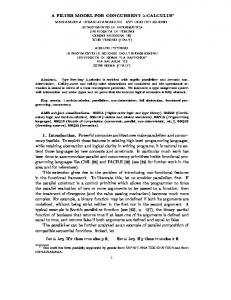
Figure 1.
A network divided into wormhole sections
As an example, consider the network in Figure 1. Each flow fi goes from its source Si to its destination Di . When a destination is shared by two flows i and j it is denoted Di,j . Let us take a closer look at f1 . f1 has to go through three wormhole sections (S1 , S2 , S4 ) to reach D1,4 with sections S1 and S4 shared with other flows. S1 and S4 are thus the two sources of direct delays for f1 . In addition, since after leaving S1 , f2 traverses section S3 which it shares with f3 , S3 will be another source of delay for f1 but only indirectly. As can be seen in this example, the wormhole section network element makes it easier to analyse the conflicts in a wormhole network. In the next section, we present a detailed model of this new network element. C. Section sharing We will present the model when there is only one interfering flow. We note f1 the studied flow. f2 is the interfering flow. fi has αiSin as an arrival curve at the entrance of section S. Let us assume that section S comprises M routers. For j = 1, . . . , M , β j is the service curve offered by the output port of router Rj to the two flows. Because of
the flow control mechanism, the amount of data which is transmitted by the port may actually be inferior to β j . Thus, β j should be seen as an intermediate parameter used to determine the service guaranteed to a given flow by this section of the network. Once we have analysed the conflicts in each output port traversed by a flow, we can use Theorem 1 to compute a service curve for the section, then for the complete path. This end-to-end curve is now valid because it takes into account the influence of all the ports used by a flow, including the indirect delays. As a consequence, it represents the real end-to-end output of the network. Since all the routers in the section are shared between the two flows and no other interference occurs, we can view these NM routers as a single router with service curve β S = j=1 β j . SpaceWire routers use a simplified Round-Robin access scheme that guarantees that each input port gets a fair acces to each output port. However, each packet can use the output port for an unlimited duration. The usual round-robin model attributes some weight to each flow and shares the bandwidth in proportion to those weights. Since the SpaceWire standard does not define such weights, we have no way of using this model and have to rely on the more pessimistic ”blind multiplexing” model [4], Theorem 6.2.1. Thus, the service curve offered by the section to f1 is M O β1S = ( β j − α2Sin )↑ .
(2)
j=1
(β)↑ is the positive and non-decreasing upper closure of β defined as (β)↑ = max(sup0≤s≤t β(s), 0). β1S is a worst-case service curve that implies that all the interfering flows have a higher priority than f1 and can instantly preempt it. Of course, in reality the packets are not interrupted but this model ensures that we have a worst-case service curve for any possible scheduling of the packets. III. S ECTION DEMULTIPLEXING A. Limits of existing models In a classic Store-And-Forward network model, the packets are instantaneously demultiplexed. Furthermore, once a packet has left the router, the delays it can endure are not propagated backward on the network. Thus, the demultiplexer has no impact on the delay (see [7] for example). However, this is not true for a wormhole network. In fact, after two flows f1 and f2 have been demultiplexed, f2 can still have an impact on f1 . This is because the
flow control mechanism will carry over the delays caused to f2 on the end of its path backward to f1 . flow control
β1
f1,α1
βτ1
f2,α2
βτ2 β2 flow control
Figure 2.
Demultiplexing of two flows in a wormhole network
A possible way to model this phenomenon is given in [8]. In this paper, the authors consider the situation described on Figure 2. In this network, after they have been demultiplexed both flows f1 and f2 have to go through a flow controller. Flow controller τi models the impact of the flow control on the downstream output link on flow fi with a service curve β τi . In turn, β τi depends on the service curve of the downstream router. The authors consider that, as far as the aggregate flow f{1,2} is concerned, τ1 and τ2 are parallel traffic regulators. As a consequence, the service offered to the aggregate flow f{1,2} is β{1,2} = min(β τ1 , β τ2 ). This aggregate service is then shared between the two flows to derive the service offered to each individual flow. This service is valid but is is very pessimistic. Let us consider the example in Figure 2. The arrival curves are affine: αi (t) = ri .t+bi and the service curves are linear: βi (t) = Ci .t We use the following values: ri (Mbps) bi (bits) Ci (Mbps)
f1 50 1000 100
f2 10 200 20
On the one hand, the service offered to f{1,2} is β{1,2} (t) = min(C1 , C2 ).t = C2 .t. On the other hand, the arrival curve of f{1,2} is α{1,2} (t) = α1 (t)+α2 (t) = r1,2 .t + b1,2 with r1,2 = r1 + r2 = 60 Mbps and b1,2 = b1 + b2 = 1200 bits. The horizontal distance h(α{1,2} , β{1,2} ) between the two curves is clearly infinite and we have to conclude that the network cannot carry both flows. This is very pessimistic because it is easy to see that this network can handle both flows. Thus we need a new, more precise network model of wormhole demultiplexer. B. A new model of demultiplexing Since both flows go in different directions in the network, we cannot determine an exact service for the
aggregated flow. Each flow receives its own service but can still cause delays to the other flow thanks to the flow control mechanism. The delay actually caused to an individual packet of f1 is hard to determine because it depends on which exact conflicts occur farther on the path of f2 . However, we can determine an upper-bound on this delay. In fact, the maximum delay caused by f2 , which we will denote d2 , is at most the maximum delivery delay from the demultiplexer to the destination of f2 . Thus, d2 =
h(α2Sout , β2dest )
(3)
where α2Sout is the arrival curve of f2 at the end of S and β2dest the service curve offered to f2 between the end of S and its destination. Here, since we have assumed a blind multiplexing with f2 as the higher priority flow, α2Sout = α2Sin
M O
βj
(4)
j=1
where (α β)(t) = sups≥0 {α(t + s) − β(s)} is the Min-Plus deconvolution of α and β. With this model, in the example in Figure 2 the delay caused by f2 to f1 is only h(α2 , β2 ) = 200 107 s = 10µs. As can be seen, this model is far less pessimistic than the model from [8]. C. Complete service curve offered by a Wormhole Section We can combine the results from Subsection II-C and III-B to obtain the complete service curve offered by section S. When two flows share Section S, the service curve offered to f1 is β1S
M O β j − α2Sin )↑ ⊗ δh(αSout ,β dest ) =( 2
(5)
2
j=1
with the delay function δT (t) = 0 if t ≤ T and δT (t) = +∞ if t ≥ T for any T ≥ 0. This formula can be easily generalized when there are more than one interfering flow. D. Computing an end-to-end service curve Once we can compute a service curve for each Wormhole Section, we have to combine them to determine an end-to-end service curve. When interfering flows arrive and depart in various routers along the path of a flow, we cannot directly use the model presented here. We would have to use a Section for each router crossed by the flow which would give us a suboptimal result. Rather, we try to optimize the ETE service curve
by combining a set of flows sharing several consecutive routers as an aggregate flow. We can then determine Wormhole Sections for this aggregate flow and deduce the service curves offered to it. Those service curves will then be shared between the individual flows composing the aggregate flow. To automate this, we plan to use the three interference patterns defined in [8] to determine the order in which the residual services are computed. IV. C ONCLUSION In this paper, we have defined a new Network Calculus element that can be used to model a SpaceWire network more accurately than the usual multiplexer and demultiplexer elements. We call this new element a Wormhole Section since it represents a part of the path followed by a flow. The Wormhole Section should allow us to obtain tighter bounds by considering successive routers as only one element. Furthermore, we also described a new way to compute the delay caused by a flow leaving a wormhole section. We showed on a simple example that our method is a lot less pessimistic than existing demultiplexer models for a wormhole network. We plan to implement a software tool based on the Wormhole Section element and the interference patterns defined in [8] to study some industrial configurations provided by Thales Alenia Space. ACKNOWLEDGMENT This work was supported by a PhD grant from the CNES and Thales Alenia Space.
R EFERENCES [1] S. M. Parkes and P. Armbruster, “Spacewire: A spacecraft onboard network for real-time communications,” IEEE-NPSS Real Time Conference, no. 14, Feb 2005. [2] ECSS, “Spacewire – links, nodes, routers and networks,” Aug 2008. [3] T. Ferrandiz, F. Frances, and C. Fraboul, “A method of computation for worst-case delay analysis on spacewire networks,” SIES ’09, 2009. [4] J. LeBoudec and P. Thiran, “Network calculus a theory of deterministic queuing systems for the internet,” Springer Verlag, no. LNCS 2050, Apr 2004. [5] F. Frances and C. Fraboul, “Using network calculus to optimize the afdx network,” ERTS 2006, Jan 2006. [6] J. L. Boudec and P. Thiran, “A short tutorial on network calculus. i. fundamental bounds in communication networks,” ISCAS 2000. [7] R. L. Cruz, “A calculus for network delay, part i: Network elements in isolation,” IEEE Transactions on Information Theory, vol. 37, no. 1, Jan 1991. [8] Y. Qian, Z. Lu, and W. Dou, “Analysis of worst-case delay bounds for best-effort communication in wormhole networks on chip,” Proceedings of the 2009 3rd ACM/IEEE International Symposium on Networks-on-Chip-Volume 00.