Using Neural Networks for Identifying Organizational Improvement Strategies
Ray Montagno Department of Management Ball State University Muncie, IN 47306
Randall S. Sexton Computer Information Systems Southwest Missouri State University 901 South National Springfield, MO 65804 USA Work: 417-836-6453 FAX: 417-836-6907 EMAIL:
[email protected] WEB: http://www.faculty.smsu.edu/r/rss000f
Brien N. Smith Department of Management Ball State University Muncie, IN 47306
1
Using Neural Networks for Identifying Organizational Improvement Strategies
Abstract The struggle to remain competitive in the global marketplace occupies much of the energy of today's firms. Although there are many performance improvement strategies that can be implemented by an organization, it has yet to be determined which strategy or combination of these strategies, if any, that is most helpful in improving performance. A genetic algorithm trained neural network is used to identify such combinations to provide direction to managers as to which performance improvement strategies are associated with increases in performance as reported by operations managers. This study shows that this neural network approach can identify combinations that result in better approximations of performance, as compared to standard statistical techniques, and should be considered as an appropriate tool for performance improvement strategy selection.
Keywords: Neural networks, strategic planning, artificial intelligence, genetic algorithms.
2
1. Introduction With the ever-increasing complexity of the global marketplace, the challenge of responding to a dynamic environment becomes paramount. Modern organizations must formulate appropriate strategies to deal with change in a timely manner. Unfortunately, the seemingly chaotic nature of the environment makes it unclear which of numerous organizational improvement strategies will work in a given context. A review of the management literature suggests that organizations have tried numerous approaches to organizational improvement. Some of these strategic approaches, like Total Quality Management (TQM), are integrative in that they encompass a broad scope of the organization (Scholtes, 1993). Other organizations attempt to use more focused approaches to improvement such as robotics or specific skills training for workers (Montagno, Ahmed and Firenze, 1995; Schonberger, 1992). One of the differences that separates the integrative from the focused approaches (Goldhar, 1985; Honeycutt et al, 1993; Kakati, 1992) is the extent to which the underlying philosophy or culture of the organization is affected by the approach used. Under the broad based approaches, it is often necessary for the organization to examine a number of its underlying values concerning control, responsibility and measurement. The difficulty in implementing these integrative approaches is that there is often considerable resistance to the change that arises in reaction to them. The focused approach (Parathasarthy and Sethi, 1993) to organizational improvement also carries with it a number of problems. Buying a sophisticated piece of equipment or providing a narrowly focused training program may have an apparent shortterm effect but in the end they may add little to organizational effectiveness. In fact, to
3
the extent that such focused programs disrupt existing processes and relationships, they may actually reduce organizational effectiveness. The existing relationships between human and material resources within a company are often complex, and such relationships are a result of considerable corporate history and evolution (March and Sproull, 1991). Attempts to make quick or poorly understood changes may lead to mediocre results for the change effort. Even broadbased approaches may yield less than desirable results when the strategy does not reflect complex organizational relationships. One research effort that has provided a framework for examining the impact of both broad based and focused organizational change is Socio-Technical-Systems (STS) analysis (Trist, 1981). The underlying assumption of STS thinking is that the social and technical aspects of an organization are separate but interdependent requirements for organizational success (Fox, 1995). The social factor generally relates to the effective use of human resources, inherently a social process. Understanding the social component involves an understanding of human needs, motivational processes, group dynamics and human learning. The technical component, on the other hand, relates to the materials, machines, territory and processes that comprise a production system. It is the smooth interface, or joint optimization, (Fox, 1995), of the two systems that leads to organizational effectiveness. One of the key features of STS, which distinguishes it from other behavioral frameworks, is the focus on the autonomous work group (Pearce and Ravlin, 1987). The use of these groups is presumed to lead to better performance and higher satisfaction. While the inclusion of groups in studies of STS has been the norm, a broader definition
4
of the social component can include all aspects of the work environment that may impact the perceptions and responses of people to their jobs. Further, the technical aspects of the work environment can be separated into two sub-categories: technical systems and technology/equipment. The first, technical systems, represents the more integrative strategies discussed above, while technology and equipment more closely resemble the focused approaches. Table 1 depicts common performance improvement strategies that are used in a socio-technical framework. (Place Table 1 approximately here) It is clear that there are a large number of operations strategies from which a firm might choose. Deciding which of these strategies, or more importantly, which combination of strategies would lead to the best organizational outcome is a question that is critical to operations managers. The research evidence on the impact of strategies has tended to focus one strategy at a time. That is, some performance dimension is identified, a change is made, and performance is measured again. Examples of studies which examine the use of single strategies include JIT (Ahmed, Tunc, and Montagno, 1991), TQM (Blest, Hunt, and Shadle. 1992) Flexible Manufacturing Systems (Vinyard, 1993), computer integrated manufacturing (Lei and Goldhar, 1990), ISO 9000 and TQM (Meegan and Taylor, 1997). Others have promoted the use of specific manufacturing technologies such as robotics, computer aided design, computer aided manufacturing, automated guided vehicles as means to reduce costs and add efficiency (Gupta and Summers, 1993). Regarding this combination of STS design practices, Majchrzak (1977) has suggested there are a number of tradeoffs in choosing one STS practice over another, and
5
that organizations rarely consider the consequences of choosing one technique over another. The selection of techniques based on time, cost, resources, or risk is often made without deference to the fact that STS practices are dependent on one another. Majchrzak points out that implementing one program but not another may actually hurt organizational effectiveness. The selection of the ideal ‘package’ of practices is highly dependent on organizational mission. Despite the evident need for studying interdependencies between STS practices, few attempts have been made to assess either the cumulative or the interactive effects of the use of STS strategies. What is needed is a procedure that will account for all possible interactions among STS practices. Then organizations could use standard cost constraints to choose the best package of techniques rather than using ‘cafeteria-style’ selection of individual techniques. One forecasting technique that may be useful in identifying such interdependence is the Neural Network. 2. Neural Networks Neural networks (NNs) represent a collection of mathematical models that provide an alternative to conventional statistical prediction techniques. While other popular techniques, such as regression, identify the linear trends in data, NNs are particularly useful in recognizing patterns in data, and abstracting the gist of input data from seemingly unrelated factors. Once the NN model has been trained on archival data, they are capable of delivering accurate predictions of future events. Neural networks have been used successfully in predicting corporate failures, and bond ratings, and have been applied in a number of applied settings including engineering and medicine.
6
3. Purpose of Study The purpose of the present study will be to investigate the usefulness of Neural Networks as a strategic tool in identifying the best pattern of improvement strategies from the Social System category (SSC) in the STS framework. Specifically, Neural Networks will be used to identify specific combinations of performance improvement strategies in the SSC that will be associated with the highest levels of performance. Additional research for the Technical System and Technology/Equipment categories will be left for future research. 3.1. Defining Performance To assess the effectiveness of SSC performance practices, a set of organizational performance indices must be chosen. Thompson and Strickland (1993) have identified the types of goals that firms usually establish to measure their success. The performance outcomes that are typically important to a firm may be classified into several categories. These goal areas relate to markets, products, economic outcomes and employees. The performance outcomes used in this study are shown in Table 2 (Place Table 2 approximately here) These performance outcomes represent an attempt to capture a broad range of outcomes that are important to firms. It could be argued that there are other outcomes that could be included in this taxonomy, however, the intent is not to create a comprehensive set of outcomes but to examine a representative set. It also can be noted that these are relatively macro outcome measures. As opposed to very specific micromeasures such as scrap rates, these measures are likely to be affected by sets of individual strategies rather than an individual activity such as a training program or a shop floor
7
LAN. While the effects of individual micro level activities are important, the focus of this research is on the grouping of these activities. 3.2. Sample There were 145 respondent firms to this survey. The firms were primarily manufacturing. The average annual sale for these firms was $101.55 million with a range of $100,000 to over $10 billion. In terms of number of employees, firms were distributed as shown in Table 3. (Place Table 3 approximately here) The size categories were determined in such way as to create groups that are approximately equal in size (except for very large firms.) Since size groupings are generally established on a convenience basis, this grouping will allow for better comparability when conducting statistical analyses. The average number of workers in each location was 235 hourly and 89 salaried workers. The average age of hourly workers was 37.87 years and of salaried workers was 41.91 years. Responding firms also represented a variety of industries. While the majority represent traditional manufacturing industries (64% from SIC codes 30-39) there are also varieties of other types of industries represented. 3.3. Survey Procedures The data for this study were collected via a mailed survey. The survey was sent with a cover letter to the chief operations manager of each firm. The letter provided instructions for completing the survey as well as highlighting the purpose of the study. Respondents were provided a preaddressed envelope in which to return the completed
8
survey. Mailing lists for the study were developed from a number of sources including the following: The Harris Directory of Industrial Firms, the membership list of the Central Indiana APICS chapter, the mailing list of the Indiana Labor and Management Council, the mailing list of the State of Delaware Productivity center, the mailing list of the Illinois Manufacturing Center. About 10,000 surveys were mailed to firms. The response rate based on 145 returns was thus 1.45%. This return rate is discussed at the end of the next section 3.4. Survey Instrument The survey is a rather lengthy document. It consists of 19 pages, broken up into 15 sections. A summary of major content areas is presented in Table 4. (Place Table 4 approximately here) Since, one of the primary thrusts of this study was to look at the current state of work and job designs, a large portion of the survey was directed at this topic. In fact, six and one half pages of the survey ask questions about work design. There are also several sections that examine human resource concerns such as desired worker characteristics, training issues, and performance appraisal. Two of the sections of the survey relate to organizational performance measurement and information reporting. The section on Breakthrough Thinking and Innovation is used as a predictor variable. It consists of nine areas that reflect underlying processes of climate within the firm. The section on performance improvement strategies was divided into three sections suing the STS model described earlier. The first section had 17 social system items, the second had 28 technical systems items, and the third had 15 technology and
9
equipment items. The last section on firm performance includes a list of outcomes on which respondents indicated how their firms have done over the last three years. There is no clear explanation for this low rate of return. The 1992 Study of Quality and Productivity Strategies used a similar strategy of distribution yet had a response rate of nearly 8% with a total return of 650 usable surveys. One difference may have been the survey itself. The details of the instrument are provided above, but compared to past surveys the current one may have been a bit more complex. For example, one of the sections required respondents to examine a work unit diagram and determine if this diagram reflected the type of work design used in their firms. This type response is at a much higher level than a typical Likert-type scale, and may have discouraged respondents from completing the survey. 4. The Genetic Algorithm The GA is a global search procedure that searches from one population of solutions to another, focusing on the area of the best solution so far, while continuously sampling the total parameter space. Research combining GAs and NNs began to appear in the mid to late 1980s. More than 250 references can readily be found in literature today (Schaffer et al., 1992). The two primary directions of this past research include using the GA to improve the performance of BP by finding optimal NN architectures and/or parameter settings, or as an alternative to BP for optimizing the network. This GA used in this study focuses on a combination of these two directions, which is the use of the GA for simultaneously finding the optimal NN architecture and optimization of the network. The NN architecture refers to the number of relevant input variables included in the final solution.
10
Most of the past research using the GA for network optimization has found that the GA is not competitive with the best gradient learning methods (Schaffer, 1994). However, it has recently been shown that the problem with this research is in the implementation of the GA and not its inability to perform the task (Sexton, Dorsey and Johnson, 1998). For example, the majority of this past research encodes each candidate solution of weights into binary strings. This approach works well for optimization of problems with only a few variables but for NNs with large numbers of weights binary encoding results in extremely long strings. As a result, the patterns (Schemas) that are essential to the GA’s effectiveness are virtually impossible to maintain with the standard GA operators such as crossover and mutation. It has been shown in empirical studies, that this type of encoding does not support any necessity, or even benefit (Davis, 1991; Michalewicz, 1992). A more effective approach is to allow the GA to operate over real valued parameters. Examples of this approach can be found in (Montana & Davis, 1989, Sexton et al., 1998). Although, Montana and Davis successfully outperformed BP using the GA, their specific implementation of the genetic algorithm resulted in the crossover operator causing excessive loss of information about the Schema of the parameters. These Schemas were influential in the prior generation selection of the current generation’s strings and therefore the loss of this information reduces the effectiveness of the search process. The alternative approach described in the Sexton et al. paper also successfully outperformed BP on a variety of problems. Unlike BP, which moves from one point to another based on gradient information, the GA simultaneously searches in many directions, which enhances the probability of
11
finding the global optimum. The following is a general description of the GA search. A formal description of the algorithm can be found in Dorsey & Mayer (1995). 4.1. Initialization Similar to BP, the GA randomly draws real values in order to begin the search. However, unlike BP, which only draws weights for one solution, the GA will draw weights for a population of solutions. The population size for this study is set to 20, which is user-defined and is based on past research (Dorsey & Mayer, 1995). Once the population of solutions is drawn, the global search begins with this first generation. 4.2. Evaluation Each of the solutions in the population is evaluated based on a pre-selected objective function, which is not necessarily differentiable. Once the solutions in the population are evaluated, a probability is assigned to each solution based on the value of the objective function. For example, the solutions that result in the smallest error terms are assigned the highest probabilities. This completes the first generation. 4.3. Reproduction The second generation is then randomly drawn from the first based on the assigned probabilities. For example, the best solutions (ones with the smallest errors and therefore highest assigned probabilities) in the first generation are more likely to be drawn for the second generation of 20 solutions. This is known as reproduction, which parallels the process of natural selection or "survival of the fittest.” The solutions that are most favorable in optimizing the objective function will reproduce and thrive in future generations, while poorer solutions die out. Before the solutions in the next generation can be evaluated, crossover and mutation operations must take place.
12
4.4. Crossover This new population, which only includes solutions that existed in the prior generation, will be randomly paired. For each pair of solutions, a random subset of weights is chosen and switched with its paired solution (crossover). For example, if a solution contains 10 weights, a random integer value is drawn from 1 to 10 for the first pair of solutions; for this example lets say 5 is selected. Every weight above the 5th weight is now switched between the paired solutions, resulting in two new solutions for each pair. 4.5. Mutation To sample the entire parameter space, and not be limited only to those initially random drawn values from the first generation, mutation must occur. Each solution in this new generation now has a small probability that any of its weights may be replaced with a value uniformly selected from the parameter space. If mutation occurs, the likelihood of this new weight surviving in the next generation is based on the probabilities assigned when the new solution is applied to the objective function. For example, if the solution now has a lower error value because of this new mutated weight, the solution containing this weight will now have a higher probability of being drawn in the next generation, or a lower probability of being drawn if it causes the error value to increase. Once replication, crossover, and mutation have occurred the new generation of solutions are evaluated to determine the new probabilities for the next generation. This process continues until the maximum number of user-defined generations (MAXGEN) has been reached. MAXGEN was set to 1,000 generations for this study. Although, this
13
value was set arbitrarily, it was found that 1,000 generations was more than sufficient for these problems. 5. Genetic Algorithm Modifications The following modifications to the GA are used to incorporate a method by which the GA can now simultaneously search for an optimal function and identify input variables that contribute to the prediction of performance. The two modifications include the objective function and mutation2, which are described in the following sections. 5.1. Objective function The SSE or RMSE is commonly used in the majority of NN research. This type of objective function is necessary because of the limitations of gradient-based search techniques, such as BP. In this study, since our criterion is to identify relevant performance improvement strategies or inputs in the model, we selected an objective function that is discontinuous as weights are added or removed. Unlike gradient-based algorithms, the GA permits this type of objective function. The specific objective function used in this study finds a solution that minimizes the sum of squared errors as well as the number of connections in the NN solution, which is shown in Equation 1. (1) N
N
E = ∑ (Oi − Oˆ i ) 2 + C i =1
∑ (O i =1
i
− Oˆ i ) 2
N
Where N is the number of exemplars in the data set, O is the output value, Ô is the NN estimate, and C is the number of non-zero weights in the solution. The penalty for any additional weight is therefore equal to the current value of the RMSE. As the optimization process gets closer to the final solution, the penalty gets smaller and
14
unnecessary weights can be eliminated. This objective function is arbitrary and was selected through trial and error. It works well for the problems in this study, but the identification of an optimal penalty is left for future research. 5.2. Mutation2 To allow the GA to identify irrelevant weights in the solutions, an additional GA operation (mutation2) was included. After mutation and before the evaluation of the new generation occurs each solution in the new generation now has a small probability that any of its weights may be replaced with a hard zero. Since the objective function penalizes for every weight that is not zero, the error will go down equal to the current RMSE for every weight that was replaced by a zero. However, the weight that was replaced might be one that the solution was depending on for a good solution, resulting in worse estimates. Based on the objective function, if the replacement causes the objective function to go down, then we can conclude that the connection was not needed for estimation, otherwise the error will grow and further generations will kill off this solution. Once replication, crossover, mutation, and mutation2 have occurred, the new generation can now be evaluated to determine the new probabilities for the next generation. 6. Experimental Design Although the STS framework has three categories of performance strategies, we chose the Social System category for this paper. The SSC includes 17 input variables. The inputs included are shown in Table 1. For example, the first input included whether or not a firm used job rotation, which was coded 0 if the firm did not use this strategy and a 1 if this strategy was used.
15
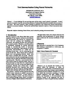
The single output used for this study included the average performance indicator scores. The 13 performance indicators, shown in Table 2, were reported by the firm with a scale of: 1=decreased, 3=remained the same, 5=increased over the past three years. Since the 7th performance indicator “lead time has” has an inverse relationship with performance, this reported outcome value was reversed before calculating the average performance for a firm. For each network, a single hidden layer was used. The number of hidden nodes for each network was determined by training the initial network with 1 hidden node and then systematically adding additional hidden nodes until the in-sample error ceased to decrease. Although, up to eight hidden nodes were tried, it was found that two hidden nodes were sufficient for finding optimal solutions. Additional hidden nodes beyond eight were not tried because further additions would cause the number weights to out number the observations in the study. Figure 1 illustrates the NN architecture for the social systems networks. (Place Figure 1 approximately here) Upon determining the number of hidden nodes for the NN, 10 replications (or NNs) were trained that only differed in the initial draw of random weights to start the training. This was done to show consistency in the algorithms ability to identify relevant input variables. The 10 networks were trained for 2,000 generations. Since eight out of the 145 responses included blank fields, these eight firms were eliminated from the three data sets, leaving 137 complete observations. Of these 137 observations, 127 observations were used for training and 10 observations were held out for testing. This was done to show that the solutions found generalized sufficiently well
16
for out-of-sample observations. Regression analysis was also conducted on these datasets to have a baseline comparison of how well the NN solutions performed compared to linear estimation techniques. 7. Results To show that the NN solutions are valid solutions, regression analysis was conducted for a baseline comparison. Regression was used on the same 127 observations that were used for the NN training. The 10 out-of-sample observations were used for testing. Two methods of regression used were ENTER and STEPWISE. The STEPWISE method only included the 13th input. The root mean squared error (RMSE) was used to compare the regression results with those of the NNs, which is shown in Table 5. Since there were 10 NN replications, the average RMSE was reported as well as the standard deviation for both in-sample and out-of-sample observations. (Place Table 5 approximately here) As can be seen by Table 5, on average, the NN outperformed regression. In fact, the NN outperformed regression in all 10 replications. To show statistical differences between those estimates that were generated by the NN solution and regression estimates, the Wilcoxon Matched Pairs Signed Ranks test was used. All comparisons were found to be significantly different at the .01 level of significance. Since we have determined that the NN found better solutions, we can now look at the combinations of performance improvement strategies that it found to be useful in predicting performance outcomes. Table 6 illustrates the number of input variables or strategies that had at least one non-zero weight in the final solution for each replication. A 1 indicates that the solution contained at least one weight connected to its respective
17
input that was non-zero. A 0 indicates that every weight connected to its respective input are zero and therefore do not contribute to the model. (Place Table 6 approximately here) The total column for Table 6, shows how many times out of 10 networks that the variable was actually used in prediction. Intuitively, if the total number was higher, the likelihood of this variable being relevant increases. By selecting a specific variable 10 times out of 10 replications, the NN is indicating that this variable contributes to its ability to produce closer estimates of the outcome variable. However, it is not clear if we should include those variables that were selected 9 times out of 10 or 8 times out of 10, etc. To specifically determine which variables to include in the model we decided that an analysis of their sensitivity should be included. This was done by creating two observations for each variable. For example, the first two observations created only differed in the value for the first input, which varied from 0 to 1 for observation 1 and 2, respectively. These two observations were then plugged into the 10 neural networks, resulting in two estimates for each network. In total, we now have 10 estimates for observation 1 and 10 estimates for observation 2. Since all other variables are held constant, varying only the first input value, we now can measure the sensitivity of changing this specific input value. The results were then compared to see the effect of changing the first input from a 0 to a 1. This was done for all 17 inputs in the problem set. Graph 1 illustrates the average sensitivity of the estimates from changing individual inputs from 0 to 1. (Graph 1 approximately here)
18
Although this graph gives us the direction of movement as well as an indication to which inputs are most significant, a test is still needed for significance. Continuing the earlier example, to test the first input for a significant change in the social system problem we took the 10 estimates where the first input was 0 (observation 1) and compared them with a t-test with the 10 estimates where the first input was 1 (observation 2). Since, the only difference between observation 1 and observation 2 was the value of the first input, we can determine from this test if the change was significant. This was done for all inputs. The variables are shown sorted by their level of significance and direction in Table 7. (Place Table 7 approximately here) Although Table 7 and Graph 1 gives us an idea of the relevance of each variable, it does so without respect to interactions that might be taking place between variables. To do this, we generated a dataset that included every possible strategy combination. For example, the first observation included zeroes for all 17 inputs. The second observation included a 1 for the first input and zeroes for the other 16 variables. This process continued until the final observation, which included 17 ones. In total, there were 131,072 possible combinations for this generated dataset. This dataset was then plugged into the 10 NNs, resulting in 131,072 performance estimates for each NN. Since each observation had 10 estimates, the average estimate was used for testing for significant differences. These average estimates were then sorted by the number of included strategies or groups. For example, there were 17 possible combinations with one variable, 136 two variable combinations, 680 three variable combinations, etc. Once this was done, we sorted by the estimate for each group of
19
combinations so we could determine which combination was best for a particular group. The sort was done in descending order since our output goal is to reach 5, the highest possible performance value. We now can determine which combination is best for each group of combinations. For example, there was 1 best combination for combinations of one variable, 1 best combination for combinations of two variables, etc. The best combination for specific group as well as their corresponding average estimate is shown in Table 8. (Place Table 8 approximately here) As can be seen in Table 8, the estimates climb in value until they peak for combinations of 12 variables. Although a 12 variable combination was shown to be the best combination overall, it is unlikely that this will often be utilized. In addition, since the estimates were close in range, we need to determine if there is a significant advantage in moving up to the next level of combinations. To do this, a t-test was conducted to see if there were statistical differences in the means of these estimates. Using the best solution and its corresponding estimate for each group of combinations, a t-test was conducted to see if there were significant differences for moving from one group of combinations to another. The results are shown in Table 9. (Place Table 9 approximately here) For example, in moving from the best one variable group to the best two variable group, the t-test was not found to be significant. However, in moving from the best one variable group to the best three variable group, the t-test was found to be significant. Therefore, if only one strategy was being implemented, there was no advantage to include only one more additional strategy, but by including two more strategies, a
20
significant difference could be found. If only two strategies were implemented, there would be no significant advantage until there were eight strategies included. However, if three strategies were going to be implemented, there was no advantage to adding any additional strategies. Obviously, many more significance tests could be conducted based on the firms situation. 8. Conclusion Although, it is not the purpose of this study to prescribe one strategy over another in all situations, it is however a place were executives can begin to examine possibilities of particular strategies and their combinations that will fit in their specific environment. It is interesting to note that the STEPWISE regression only included 13th variable but the NN found that if only 1 variable or strategy is to be used the 11th strategy is the best. This may have occurred because of the interactions that take place between strategies. The NN models did however include the 13th variable in every other best solution for each group of combinations. One obvious limitation to this study is the limited number of observations collected for neural network analysis. Future research is needed that will include many more observations in order to validate the outcomes of this study. Other possible areas of future research include the prediction of specific performance areas as shown in Table 2 as well as the other two categories of strategies from the STS model. The neural network model has been shown to predict well in many areas of business. By incorporating the genetic algorithm and its modifications, user’s are better able to identify relevant variables in a model, which in turn, help the user make decisions that were in the past based only on intuition.
21
References: Ahmed, N.U., E.A. Tunc, and R. V. Montagno. “A comparative Study of U.S. Manufacturing Firms in Various Stages of Just-in-Time Implementation.” International Journal of Production Research 29, no. 4 (1991): 787-802. Blest, J. P., R. G. Hunt, and C. C. Shadle. “Action Teams in the Total Quality Process: Experience in a Job Shop.” National Productivity Review (spring 1992): 195-202. Davis, L. (ed.) (1991). Handbook of Genetic Algorithms, Van Nostrand Reinhold, NY. Dorsey, R. E. & Mayer W. J., (1995). Genetic algorithms for estimation problems with multiple optima, non-differentiability, and other irregular features. Journal of Business and Economic Statistics, 13(1), 53-66. Dorsey, R. E., Johnson, J. D. & Mayer, W. J. (1994). A genetic algorithm for the training of feedforward neural networks. Advances in Artificial Intelligence in Economics, Finance, and Management (J. D. Johnson and A. B. Whinston, eds., 93-111). Vol. 1. Greenwich, CT: JAI Press Inc. Dorsey, R. E., Johnson, J. D. & Van Boening, M. V. (1994). The use of artificial neural networks for estimation of decision surfaces in first price sealed bid auctions. In W.W. Cooper and A.B. Whinston (eds.), New Direction in Computational Economics (pp. 1940). Netherlands:Kluwer Academic Publishers. Fox, W. M. (1995). Sociotechnical system principles and guidelines: Past and present. Journal of Applied Behavioral Science, 31(1), pp. 91-106. Goldhar, J.D., “Computer integrated flexible manufacturing: organizational, economic, and strategic implications”, Interfaces, Vol. 15 No. 3, 1985, pp. 94-105. Gupta, Y. P., and T, M. Summers. “Factory Automation and Integration of Business Function.” Journal of Manufacturing Systems 12, no.1 (1993): 58-61. Honeycutt, A. (1993). Total Quality Management at TRW. Journal of Management Development, 12( 5), p0-0.
22
Kakati, M. (1992). Prescriptive model for organizing and managing FMS and CIM environment. Human Systems Management, 11(4), pp. 193-202. Lei, D., and J. D. Gjoldhar. “Multiple Niche Competition: The Strategic Use of CIM Technologies.” Manufarturing Review 3, no. 3 (1990):195-206. Majchrzak, A. (1997). What to do when you can't have it all: Toward a theory of sociotechnical dependencies. Human Relations, 50(5), pp. 535-566.
March, J. G., Sproull, L. S., & Tamuz, M. (1991). Learning from samples of one or fewer. Organizational Science, 2(1), 1-13. Meegan, Sarah T. and Taylor, W. Andrew. “Factors influencing a successful transition from ISO 9000 to TQM: The influence of understanding and motivation.” International Journal of Quality & Reliability Management, Vol. 14 No. 2, 1997, pp. 100-117. Michalewicz, Z. (1992). Genetic Algorithms + Data Structures = Evolution Programs. Springer, Berlin. Montagno, Ray V., Ahmed, Nazim H., and Firenze, Robert J., “Perceptions of Operations Strategies and Technologies in U.S. Manufacturing Firms”, Production and Inventory Management Journal, Vol. 36, #2, Second Quarter 1995, pp. 22-27. Montana, D. J. & Davis, L. (1989). Training feedforward neural networks using genetic algorithms. Proceedings of the Third International Conference on Genetic Algorithms, Morgan Kaufmann, San Mateo, CA, 379-384. Parathasarthy, R. & Sethi, S.P. (1992). The impact of flexible automation on business strategy and organizational structure, Academy of Management Review, 17, pp. 86-111. Pierce, J. A., & Ravlin, E. C. (1987). The design and activation of self-regulating work groups. Human Relations, 40, 751-782. Schaffer, J. D., Whitley, D., & Eshelman, L. J. (1992). Combinations of genetic algorithms and neural networks: A survey of the state of the art, COGANN-92. Combinations of Genetic Algorithms and Neural Networks (pp. 1-37). IEEE Computer Society Press, Los Alamitos, CA. Schaffer, J. D. (1994). Combinations of genetic algorithms with neural networks or fuzzy systems. Computational Intelligence: Imitating Life (pp. 371-382). J.M. Zurada, R.J. Marks, and C. J. Robinson, eds., IEEE Press. Scholtes, P. R. (1993). Total quality or performance appraisal: Choose one. National Productivity Review, 12(3), pp. 349-364.
23
Schonberger, R.J., “Is strategy strategic? Impact of total quality management on strategy”, Academy of Management Executive, Vol. 6, August 1992, pp. 80-7. Sexton, R. S., Dorsey, R. E., & Johnson, J. D. (1998). Toward a global optimum for neural networks: a comparison of the genetic algorithm and backpropagation. Decision Support Systems, 22, 171-185. Thompson, A. A. and Strickland, A.J., Strategic Management, 7th ed., Irwin, Burr Ridge, IL, 1993, pp. 20-54. Trist, E. (1981). The sociotechnical perspective. In A. Van de Ven & W. Joyce (Eds.), Perspectives in organizational design and behavior (pp. 203-221). New York: Wiley. Vinyard, M. L. “FMS Performance: A Long-Term Study.” Production and Inventory Management Journal 34, no.2(1993): 38-42.
24
25
Table 1 – Performance Improvement Strategies Social System Category (SSC) 1. Job rotation 2. Multi-skill training 3. Cross-functional problem solving groups 4. Self-directed work teams 5. Intradepartmental problem solving groups 6. Team/group performance appraisal 7. Pay for knowledge (skill-based pay) 8. Profit sharing 9. Four-day work week 10. Flextime 11. Company paid child care 12. Wellness program 13. Hourly people involved with selecting and implementing technology 14. Hourly people involved with design of work 15. Supervisor training for group-based work 16. Part-time workers 17. Temporary workers
26
Table 2 –Performance Outcomes 1. Degree of market share 2. Overall sales volume 3. Product/service quality 4. New and improved product introductions 5. Productivity 6. Profitability 7. Lead times 8. Organization’s capacity to use appropriate technology 9. Product value to customer 10. On-time delivery 11. Ability to meet customer cost requirements 12. Ability to provide customized products/services 13. Ability to penetrate new markets
27
Table 3 – Company Size Distribution Number of Number of Employees Companies 0-50 36 51-100 36 101-200 30 201-1000 33 1001 + 8
28
Table 4 – Major Content Areas of Survey Content Area Firm Demographics CEO Concerns Work Designs and Work Characteristics Worker Characteristics Welfare to Work Training and Appraisal Systems Performance Measurement and Reporting Breakthrough Thinking and Innovation Performance Improvement Strategies Firm Performance
29
Figure 1 – Typical Social System Neural Network
Output
Hidden
Inputs
30
Table 5 – RMSE Comparison Social System NN Enter In-Sample 0.41 0.43 Holdout 0.36 0.44 In-Stdev 0.01 N/A Out-Stdev 0.06 N/A
Step 0.44 0.41 N/A N/A
31
Table 6 – Relevant Input Variables Replication 1 Input 1. Job rotation 1 2. Multi-skill training 1 3. Cross-functional problem solving groups 0 4. Self-directed work teams 0 5. Intradepartmental problem solving groups 1 6. Team/group performance appraisal 0 7. Pay for knowledge (skill-based pay) 1 8. Profit sharing 1 9. Four-day work week 1 10. Flextime 1 11. Company paid child care 0 12. Wellness program 1 13. Hourly people involved with selecting 1 and implementing technology 14. Hourly people involved with design of 1 work 15. Supervisor training for group-based 0 work 16. Part-time workers 1 17. Temporary workers 1 * = Best RMSE for in-sample and out-of-sample
2
3
4
5
6
8
9
10
Total
1 1 0 0 0 0 0 1 1 1 1 1 1
7 * 0 1 1 1 1 0 1 1 1 1 1 1 1
1 0 1 1 0 0 1 1 1 1 1 1 1
1 1 0 0 1 0 1 1 1 1 0 1 1
1 1 0 0 1 0 1 1 1 1 0 1 1
1 0 1 0 0 0 0 0 1 1 0 1 1
1 0 0 1 1 1 0 0 1 1 1 1 1
0 1 0 0 0 0 1 0 1 1 0 1 1
0 1 1 0 1 1 0 0 1 1 1 1 1
7 7 4 3 6 2 6 6 10 10 5 10 10
1
1
1
1
1
1
1
0
1
9
1
0
0
1
1
1
0
0
1
5
0 0
1 1
1 1
0 1
1 1
0 1
1 1
1 1
1 1
7 9
32
Graph 1
Social System Variable Sensitivity 0.3 0.2
Sensitivity
0.1 0 -0.1
1 2 3 4 5 6 7 8 9 10 11 12 13 14 15 16 17
-0.2 -0.3 -0.4 Variables
Series1
33
Table 7—Variable Significance Social System Variable P-Value Direction 13 0.007 + 10 0.050 + 11 0.061 + 1 0.221 + 2 0.237 + 14 0.584 + 7 0.621 + 4 0.767 + 6 0.777 + 9 0.003 12 0.048 17 0.097 16 0.474 3 0.746 15 0.783 8 0.937 5 0.976 -
34
Table 8 – Best Combination by Group of Combinations Variable 1 2 3 4 5 6 7 8 9 10 11 Group 0 0 0 0 0 0 0 0 0 0 0 1 0 0 0 0 0 0 0 0 0 0 1 2 0 0 0 0 0 0 0 0 0 0 1 3 0 0 0 0 0 0 0 0 0 1 1 4 0 0 0 0 0 0 1 0 0 1 1 5 0 0 1 0 0 0 1 0 0 1 1 6 0 0 1 1 0 0 1 0 0 1 1 7 0 1 1 0 0 0 1 0 0 1 1 8 1 0 1 0 1 0 1 0 0 1 1 9 1 0 1 0 1 0 1 0 0 1 1 10 1 1 1 0 1 0 1 0 0 1 1 11 1 1 1 0 1 0 1 0 0 1 1 12 1 1 1 1 1 0 1 0 0 1 1 13 1 1 1 1 1 1 1 0 0 1 1 14 1 1 1 1 1 1 1 1 0 1 1 15 1 1 1 1 1 1 1 1 0 1 1 16 1 1 1 1 1 1 1 1 0 1 1 17 1 1 1 1 1 1 1 1 1 1 1
12 0 0 0 0 0 0 0 0 0 0 0 0 0 0 0 1 1 1
13 0 0 1 1 1 1 1 1 1 1 1 1 1 1 1 1 1 1
14 0 0 0 0 0 0 0 0 1 1 1 1 1 1 1 1 1 1
15 0 0 0 0 0 0 0 0 0 1 0 1 1 1 1 1 1 1
16 0 0 0 0 0 0 0 1 0 0 1 1 1 1 1 1 1 1
17 0 0 0 0 0 0 0 0 0 0 0 0 0 0 0 0 1 1
Est. 3.86 4.19 4.43 4.59 4.63 4.65 4.65 4.67 4.72 4.73 4.75 4.76 4.76 4.73 4.70 4.62 4.52 4.33
35
Table 9 – Significant Estimate Change 0 1 2 3 4 5 6 7 8 9 10 11 12 13 14 15 16 17 0 1 * 2 * 3 * * 4 * * 5 * * 6 * * 7 * * 8 * * * 9 * * * 10 * * * 11 * * * 12 * * * 13 * * * 14 * * * 15 * * 16 * * 17 * * * * * * * * * * * * * * = significant change in the average estimates