Using nonisochronicity to control synchronization in ensembles of ...

CHAOS

VOLUME 13, NUMBER 1

MARCH 2003

Using nonisochronicity to control synchronization in ensembles of nonidentical oscillators Ernest Montbrio´ and Bernd Blasius Institut fu¨r Physik, Universita¨t Potsdam, Postfach 601553, D-14415 Potsdam, Germany

共Received 23 May 2002; accepted 30 September 2002; published 21 February 2003兲 We investigate the transition to synchronization in ensembles of coupled oscillators with quenched disorder. We find that small coupling is able to increase the frequency disorder and to induce a spread of oscillator frequencies. This new effect of anomalous desynchronization is studied with numerical and analytical means in a large class of systems including Ro¨ssler, Lotka–Volterra, Landau–Stuart, and Van-der-Pol oscillators. We show that anomalous effects arise due to an interplay between nonisochronicity and natural frequency of each oscillator and can either increase or inhibit synchronization in the ensemble. This provides a novel possibility to control the synchronization transition in nonidentical systems by suitably distributing the disorder among system parameters. We conjecture that our results are of relevance for biological systems. © 2003 American Institute of Physics. 关DOI: 10.1063/1.1525170兴

and the frequency differences of the oscillators. Of special interest is the phenomenon of phase synchronization in which coupling can overcome the dispersal of natural frequencies and the oscillators mutually adjust their frequencies to a common locking frequency.3 Phase synchronization is a ubiquitous phenomenon and arises naturally in many areas of physics and living systems. It appears in pairs of mutually coupled limit cycle systems and in phase coherent chaotic oscillators.4 But phase synchronization is also dominant in systems of many interacting oscillators and has been demonstrated in one- or two-dimensional lattices and in large sets of globally coupled limit cycle systems2,5–10 and chaotic oscillators.11–13 Biological examples of such synchronization phenomena include synchronous flashing fireflies,14 firing of neurons and neural networks,15,16 the cardio-respiratory system,17 and oscillating population numbers.18,19 Usually the introduction of coupling simply leads to synchronization between the oscillators. However, coupling may also give rise to a plethora of different effects including oscillation death,8,20,21 desynchronization in a short-wavelength bifurcation22 or dephasing with bursts of amplitude change.23,24 In this paper, we present a novel mechanism for coupling induced desynchronization. We focus on an ensemble of oscillators under the presence of quenched noise and systematically investigate the effects of weak coupling on the frequency distribution between the oscillators. We report on an unusual transition to synchronization where coupling can enlarge the natural disorder of frequencies and desynchronize the whole ensemble of oscillators.31 This new phenomenon is explored with numerical simulations and by analytical means. We are able to demonstrate that anomalous synchronization originates in the nonisochronicity of oscillation and arises when nonisochronicity increases with the natural frequency of oscillation. On the other hand when nonisochronicity and natural frequency have negative covariance synchronization can be dramatically enhanced. This opens the door for the possibility of synchronization control; with a careful choice of oscillator parameters the effect of

The study of synchronization phenomena in populations of interacting oscillators has been a broad and promising field of research in the last decades with many applications in a large class of systems. In any real application the oscillators are necessarily nonidentical and vary in their system parameters. Such natural disorder is always present, for example, in biological oscillators and reflects the natural heterogeneity of any living environment. Usually, in studies of disordered ensembles of oscillators the disorder is realized by variations in only one variable. Here, we demonstrate that unusual properties arise when disorder is affecting two characteristics of the system simultaneously. In our case, parameter mismatch between different oscillators has influence both on the natural frequency and on the nonisochronicity of oscillation. This is a realistic assumption in many natural systems and mathematical models. Under these assumptions we show a new phenomenon where coupling counterintuitively can desynchronize the ensemble of oscillators. We denote this novel effect as ‘‘anomalous synchronization.’’ It appears when nonisochronicity covaries with the natural oscillator frequency. The effect of anomalous synchronization allows us to control the transition to synchronization and also the synchronization threshold. Therefore, it is of potential use for engineering applications, but also should play a role in living systems where evolution may have selected parameter sets in such a way as to support biologically advantageous synchronization properties. I. INTRODUCTION

The study of coupled oscillator systems is one of the most fundamental problems in nonlinear dynamics and is of considerable importance in a variety of physical and biological applications.1,2 In practice it is inevitable that the oscillators are nonidentical and vary in their natural frequencies. Synchronization then arises as an interplay between coupling 1054-1500/2003/13(1)/291/18/$20.00

291

© 2003 American Institute of Physics

Downloaded 30 Sep 2005 to 193.145.45.239. Redistribution subject to AIP license or copyright, see http://chaos.aip.org/chaos/copyright.jsp

292

E. Montbrio´ and B. Blasius

Chaos, Vol. 13, No. 1, 2003

anomalous synchronization can be used to either enhance or inhibit the synchronization in the ensemble. Similar strategies can easily be used in biological systems and thus anomalous synchronization might play an important role in living systems. The outline of the paper is as follows: first, to set the framework in Sec. II we define the type of systems under investigation as an interacting ensemble of limit cycle systems or chaotic oscillators. Further, we review some basic properties of phase synchronization in such systems. Next, we use these methods to numerically explore the transition to phase synchronization in spatially extended ecological systems with oscillating dynamics. This will lead us to the phenomenon of anomalous phase synchronization 共Sec. III兲. In Sec. IV we present some analytic arguments which demonstrate the origin of these effects and provide exact criteria when anomalous effects are to be expected. To show that anomalous synchronization appears universally, in Sec. V we go over to coupled Landau–Stuart models and phase equations. There, we identify the effect as a consequence of the nonisochronicity of oscillation. This allows to develop a full analytic description of the transition to synchronization in two coupled phase oscillators. Finally, using the example of weakly nonlinear Van-der-Pol oscillators we show that the theoretical results can effectively be applied for the control of the transition to synchronization 共Sec. VI兲. In Sec. VII we summarize our results and speculate on the possible relevance for biological systems.

II. A SHORT PRIMER OF PHASE SYNCHRONIZATION

In this paper we study the synchronization properties in a system of N coupled nonidentical oscillators of the following type: m

x˙i⫽F共 xi ; ␹ i 兲 ⫹

⑀ C 兺共 xj⫺xi兲 , m j⫽1

i⫽1,...,N.

共1兲

To be more specific the systems under investigation obey the following properties: 共a兲

共b兲

In the absence of coupling each oscillator follows its own local dynamics x˙⫽F(x, ␹ ), where x苸Rn . All oscillators have the same functional form but depend on a set of l control parameters ␹ ⫽(a,b,...). We always assume that each oscillator is parameterized either on a limit cycle or on a regime with phase coherent chaos. Thus every, possibly chaotic, oscillator is characterized by a well defined natural frequency which is given by the long term average of phase velocity, ␻ ⫽¯␪˙ (t). 3 Disorder or quenched noise is imposed onto the system by assigning to each oscillator i an independent value for every control parameter out of the set ␹ i , usually taken from a statistical distribution. Here, we always use a uniform distribution. However our results remain valid if different distributions such as a Gaussian are used. In general, the control parameters affect the natural or unperturbed frequency of each oscillator, ␻ i ⫽ ␻ ( ␹ i ). Therefore, the natural disorder in control pa-

共c兲

rameters leads to a frequency mismatch between the oscillators which we also refer to as frequency disorder. Each oscillator is coupled with strength ⑀ to a predefined set of m neighbors 兵 j 其 . In this paper, we consider only two cases: either coupling to next neighbors in a one- or two-dimensional lattice or global coupling. However we have obtained similar results with different coupling topologies. C⫽diag(c1 ,c2 ,. . . ,cn) is a diagonal matrix which indicates the strength of the interaction in each component of the state vector x. We also assume that even with the onset of coupling each oscillator is still rotating uniformly. This means especially that we do not allow for situations with oscillation death.8,9,20,21 In practice, this can always be realized if the coupling is restricted to be small enough.

Synchronization arises as an interplay between the interaction and the frequency mismatch of the oscillators. Thereby, in general, the frequency of each oscillator will be detuned ⍀ i ⫽⍀ i 共 ⑀ 兲 .

共2兲

We denote the oscillator frequency in the presence of coupling with a capital ⍀共⑀兲 in contrast to the natural frequency ␻ of the uncoupled oscillator, e.g., ␻ ⫽⍀(0). Phase synchronization refers to the fact that with sufficient coupling strength ⑀ ⬎ ⑀ c all oscillators rotate with the same frequency, ˜ . This definition is used as our main criterion to detect ⍀ i ⫽⍀ phase synchronization throughout in this paper. Beside the original system 共1兲 we sometimes use an alternative framework to describe the system dynamics. This is possible since we have assumed that each oscillator is rotating uniformly and therefore it’s 共uncoupled兲 dynamics can be described in terms of phase variables ␪˙ i ⫽ ␻ i . In the case of weakly coupled, nearly identical oscillators, the long-term dynamics of system 共1兲 is given by phase equations of the following form:2,5,21,25

␪˙ i ⫽ ␻ i ⫹

⑀ ⌫ i j共 ␪ j⫺ ␪ i 兲. m兺 j

共3兲

In this equation, the interaction function ⌫ i j represents the effects of coupling and, in general, is a 2␲-periodic function of the phase difference between the interacting oscillator pairs, ⌬ ␪ ⫽ ␪ j ⫺ ␪ i . It can be calculated from the original system as the following integral:2 ⌫ i j共 ⌬ ␪ 兲⫽

1 2␲

冕

2␲

␾ ⫽0

Z i 共 ␾ 兲 p i j 共 ␾ ,⌬ ␪ 兲 d ␾ .

共4兲

Here, the sensitivity vector Z i ( ␾ ) describes the phase shift that is induced in oscillator i after a perturbation at phase ␾, and p i j ( ␾ , ␦ ␪ ) describes the perturbation of the state of oscillator i with phase ␾ due to the interaction with another oscillator j of phase ␾ ⫹⌬ ␪ . The simplest form of the coupling function arises as the first term in a Fourier expansion of ⌫ i j (⌬ ␪ ) 共Kuramoto model兲,2 ⌫ 共 ␪ j ⫺ ␪ i 兲 ⫽sin共 ␪ j ⫺ ␪ i 兲 .

共5兲


Chaos, Vol. 13, No. 1, 2003

Nonidentical oscillators

293

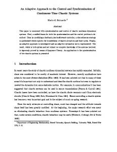
FIG. 1. Synchronization of two simple phase oscillators 共6兲. Plotted is the frequency difference ⌬⍀( ⑀ ) 共left兲 and the frequencies of each oscillator ⍀ 12( ⑀ ) 共right兲 as a function of coupling strength, ⑀.

We now investigate the mutual entrainment of two nonidentical phase oscillators which are coupled according to 共5兲

␪˙ 1 ⫽ ␻ 1 ⫹ ⑀ sin共 ␪ 2 ⫺ ␪ 1 兲 , ␪˙ 2 ⫽ ␻ 2 ⫹ ⑀ sin共 ␪ 1 ⫺ ␪ 2 兲 .

共6兲

The transition to synchronization is depicted in Fig. 1. Both oscillators start out with a natural frequency difference ⌬ ␻ ⫽ ␻ 2 ⫺ ␻ 1 . With the onset of interaction both oscillator frequencies are detuned 共2兲 and are attracted towards each other. Finally, in the synchronized state, they collide to the ˜ ⫽( ␻ 1 ⫹ ␻ 2 )/2. The transition to synchrosingle frequency ⍀ nization can be visualized through a plot of the frequency difference ⌬⍀( ⑀ ) which is a monotonically decreasing function of coupling. When the coupling exceeds a critical value, ⑀ ⬎ ⑀ c , the frequency difference disappears ⌬⍀( ⑀ )⫽0 and the oscillators are synchronized to a common frequency. It is also possible to describe the process of synchronization in system 共6兲 analytically. Subtraction of both equations in 共6兲 leads to a single equation for the phase difference, ⌬ ␪˙ ⫽⌬ ␻ ⫺2 ⑀ sin共 ⌬ ␪ 兲 ,

共7兲

which can simply be integrated to obtain the phase difference as a function of coupling 共see, for example, Ref. 33兲. This leads to the well known beat frequency of two coupled phase oscillators ( ⑀ ⬍⌬ ␻ /2), ⌬⍀ 共 ⑀ 兲 ⫽ 冑⌬ ␻ 2 ⫺4 ⑀ 2 .

共8兲

When the coupling exceeds the synchronization threshold ⑀ c ⫽⌬ ␻ /2, then ⌬ ␪˙ ⫽0 and the phases of both oscillators are related by a fixed phase difference sin(⌬␪)⫽⌬␻/(2⑀). Thus, for small coupling levels the state of the system is characterized by the frequency difference ⌬⍀( ⑀ ). With the onset of synchronization the frequency difference disappears and the state of the system can be characterized by the phase lag ⌬ ␪ ( ⑀ ). Strictly speaking this gives rise to two independent definitions of synchronization. The fact that the phase difference in the synchronized state is bounded, 兩 ⌬ ␪ (t) 兩 ⬍const, is called phase locking or phase synchronization. In contrast, the fact that the frequency difference disappears, ⌬⍀⫽0, is referred to as frequency synchronization. The difference between these two definitions becomes important in stochastic

systems.3 For the purpose of this article, however, this distinction plays no role, and from now on we simply denote both phenomena as phase synchronization. The process of synchronization in two mutually coupled phase oscillators as described above is particularly simple. It is known for long time that similar phenomena occur if two limit cycle systems are coupled.3 Interestingly, these ideas can directly be extended to systems with self-sustained chaotic dynamics.4 For these aims it is necessary to extend the concepts of phase and frequency to the case of a chaotic attractor. This is well established in phase coherent chaotic systems. Take for example the Ro¨ssler system,26 x˙ ⫽⫺by⫺z,

y˙ ⫽bx⫹ay,

z˙ ⫽0.4⫹ 共 x⫺8.5兲 z.

共9兲

In the parameter range a⬇0.15 and b⬇1 the motion shows phase coherent dynamics 共see also Fig. 4兲. In this regime a phase can be defined as an angle in (x,y)-phase plane or via the Hilbert-transform.4 In this paper, we always estimate the phase of chaotic systems by counting successive maxima, e.g., we locate the times t n of the n th local maxima of the y-variable. We define that the phase increases by 2␲ between two successive maxima and interpolate linearly in between3

␾ 共 t 兲 ⫽2 ␲

t⫺t n ⫹2 ␲ n, t n⫹1 ⫺t n

t n ⬍t⬍t n⫹1 .

共10兲

Now we explore the transition to synchronization in two mutually coupled Ro¨ssler systems 共see Fig. 2兲. The oscillators are nonidentical and vary in the value of parameter b. Both oscillators are diffusively coupled in the y variable with strength ⑀ 关e.g., by adding the term ⑀ (y 2,1⫺y 1,2) in the equation of y˙ 1,2]. As can be seen in Fig. 2 despite the chaotic amplitudes the transition to the synchronized state is very similar to the case of two coupled phase oscillators. Due to the interaction both oscillators are detuned and the frequencies approach each other. As a result the frequency difference, ⌬⍀( ⑀ ) decreases monotonically until it becomes zero in the synchronized state. In the following we study how these ideas generalize to an ensemble of many interacting Ro¨ssler systems12 x˙ i ⫽⫺b i y i ⫺z i , y˙ i ⫽b i x i ⫹ay i ⫹

⑀ 共 y j ⫺y i 兲 , m兺 j

共11兲

z˙i ⫽0.4⫹ 共 x i ⫺8.5兲 z i .


294


Chaos, Vol. 13, No. 1, 2003

FIG. 2. Transition to synchronization in two coupled Ro¨ssler systems 共9兲. Plotted is the frequency difference ⌬⍀( ⑀ ) 共left兲 and the individual frequencies of each oscillator, ⍀ 12( ⑀ ) 共right兲 as a function of coupling strength. Parameter values a⫽0.15, b 1,2⫽1.0⫾0.01.

Here, all Ro¨ssler oscillators are nonidentical. The disorder is realized by taking the parameters b i for each oscillator from a uniform distribution and thereby assigning it its own frequency ␻ i ⬇b i . In Fig. 3 we plot the numerical results in a ring of ten locally coupled Ro¨ssler oscillators. With the onset of coupling the frequencies of all oscillators move towards each other forming synchronized clusters. At a certain coupling strength only one cluster is left and the ensemble has reached the synchronized state. A convenient measure to characterize the amount of frequency disorder is the standard deviation of all oscillator frequencies ␴ ( ⑀ ). As is demonstrated in Fig. 3, ␴ ( ⑀ ) is a decreasing function of coupling strength. Global phase synchronization is achieved when ␴ ( ⑀ ⬎ ⑀ c )⫽0 and all oscillators rotate with the same frequency. By comparing Fig. 3 with Figs. 1 and 2 it follows that in interacting oscillator systems the standard deviation ␴ ( ⑀ ) takes over the role of ⌬⍀( ⑀ ) in the case of two coupled oscillators. Another frequently used measure to characterize the amount of synchronization in large populations of oscillators is the complex order parameter z. It can be obtained by summing up the phases ␪ j of all oscillators in the complex plane, 1 z⫽Re ⫽ N i⌿

N

兺

j⫽1

i␪ j

e .

共12兲

The order parameter R is given by the amplitude of z and ⌿ defines the average phase in the ensemble.2 In contrast to the frequency disorder ␴ the order parameter R does not provide direct information about the oscillator frequencies. Instead it

reflects the average positions of the oscillators on their trajectories in the unit circle. Therefore, the order parameter is an excellent measure for the detection of clustering in the ensemble of oscillators. Without coupling all oscillators rotate independently on the unit circle and the order parameter is nearly zero, R⬃1/冑N. In contrast when the ensemble is synchronized all oscillators rotate coherently and R→1. Note, that R can be obtained from a snapshot of the oscillator phases at a single instant in time. In contrast, the calculation of the frequency disorder, ␴, is more involved since the time evolution of every oscillator has to be followed. To summarize, in order to measure the transition to synchronization in a system of interacting oscillators 共1兲 we identify the frequency of each oscillator in dependence of the coupling strength, ␻ i ( ⑀ ). For phase coherent chaotic dynamics this is done by counting the number of local maxima of a chosen variable. We define the frequency disorder as the standard deviation of all oscillator frequencies ␴ ( ⑀ ). Then synchronization is given by the single criterion that ␴ ( ⑀ ) ⫽0. Occasionly, we also use the complex order parameter R( ⑀ ) to characterize the synchrony in the ensemble which then is always compared to our usual measure. III. ANOMALOUS SYNCHRONIZATION IN ECOLOGICAL MODELS

The question arises whether the simple transition to synchronization as exemplified in Figs. 1, 2, and 3 is universal, e.g., whether the frequency disorder ␴ ( ⑀ ) is always a monotonically decreasing function of coupling strength. To explore this case we turn to spatially extended ecological sys-

FIG. 3. Transition to synchronization in a ring of ten diffusively coupled Ro¨ssler systems 共11兲 with periodic boundary conditions. Plotted is the standard deviation ␴ ( ⑀ ) of all oscillator frequencies in percent 共left兲 and the individual oscillator frequencies ⍀ i 共right兲 as a function of coupling strength ⑀. Parameters are taken randomly in the range b i ⫽0.97⫾0.025 and a⫽0.15.


Chaos, Vol. 13, No. 1, 2003


295

FIG. 4. Comparison of the transition to synchronization in a chain of 500 locally coupled Ro¨ssler systems 共11兲共left兲 and foodweb models 共13兲共right兲. Oscillators have been coupled in the y-variable with strength ⑀ to next neighbors in a ring with periodic boundary conditions. Inital values were set randomly. Top: attractor projection of the uncoupled system in the (x,y)-plane. Bottom: standard deviation of frequencies, ␴ ( ⑀ ), as a function of coupling strength. Parameter values: Ro¨ssler system a⫽0.15. Foodweb model x 0 ⫽1.5, y 0 ⫽0, z 0 ⫽0.1, ␣ 1 ⫽0.1, ␣ 2 ⫽0.6, a⫽1, c⫽10. Parameters b i are taken in both systems as uniformly distributed random numbers in the range b i ⫽0.97⫾0.025.

tems which are examples for spatio-temporal synchronization in natural systems.27 Maybe the most intriguing example is Ecology’s well known Canadian harelynx cycle with hare and lynx populations synchronizing in phase to a collective 10-year cycle over the entire Canadian Continent.19,28,30 In order to describe such phenomenon the following model has been proposed:13,19 x˙ i ⫽a 共 x i ⫺x 0 兲 ⫺ ␣ 1 x i y i , y˙ i ⫽⫺b i 共 y i ⫺y 0 兲 ⫹ ␣ 1 x i y i ⫺ ␣ 2 y i z i ⫹

⑀ m

兺j 共 y j ⫺y i 兲 , 共13兲

z˙ i ⫽⫺c 共 z i ⫺z 0 兲 ⫹ ␣ 2 y i z i . This model describes a three level ‘‘vertical’’ food chain where the vegetation x is consumed by herbivores y which themselves are preyed upon by the top predator z. In the absence of interspecific interactions the dynamics is linearly expanded around the steady state (x 0 ,y 0 ,z 0 ) with coefficients a, b, and c that represent the respective nett growth and death rates of each species. Predator–prey interactions are introduced via Lotka–Volterra terms with strength ␣ 1 and ␣ 2 . Despite their minimal structure, the equations are able to capture complex dynamics which matches real data for example in the Canadian hare-lynx cycle.13,19,29,30 In this parameter range the model shows phase coherent chaotic dynamics, where the trajectory rotates with nearly constant frequency in the (x,y)-plane but with chaotic dynamics that appear as irregular spikes in the top predator z 共Fig. 4兲. This

behavior of the foodweb model is reminiscent to the Ro¨ssler system 共11兲 and therefore one might expect similar synchronization properties in both systems. To explore this in more detail, in Fig. 4 we compare the transition to synchronization in coupled chains of Ro¨ssler and foodweb systems. Quenched disorder is introduced by taking b i for each oscillator from the same statistical distribution. Despite the fact that both systems have very similar attractor topology we find fundamental differences in their response to the interaction. For the ensemble of Ro¨ssler systems the onset of synchronization is as expected and ␴ ( ⑀ ) decreases monotonically with increasing coupling strength, in accordance to the above theory. In contrast, the ensemble of foodweb models shows a totally different behavior. Here, with increasing coupling the frequency disorder is first amplified leading to a maximal decoherence for intermediate levels of coupling. Only for much larger coupling strength frequency disorder is reduced again and synchronization sets in. We denote this unusual increase of disorder with coupling strength as anomalous transition to phase synchronization.31 We have tested the robustness of anomalous synchronization in a large number of numerical simulations. We have always found that the long term behavior is independent of initial conditions, which usually are set randomly for each oscillator 共in the foodweb model initial conditions have to be taken out of the domain of attraction of the phase coherent attractor兲. Our results are numerically robust to the network topology. We have numerically checked simulations in oneand two-dimensional lattices with different sizes and also in systems with global coupling. In all cases we have found large parameter ranges in which the ecological model exhibits anomalous synchronization 共Fig. 5兲. In general, the


296

Chaos, Vol. 13, No. 1, 2003

E. Montbrio´ and B. Blasius FIG. 5. Onset of synchronization in a chain of 500 nonidentical Ro¨ssler systems 共11兲共left兲 and foodweb models 共13兲共right兲 for different coupling topologies. Plotted is the standard deviation of frequencies, ␴ ( ⑀ ). Oscillators are coupled in the y-variable with strength ⑀ either in a ring with next neighbor coupling 共solid lines兲, with global coupling 共dashed lines兲 or using the approximation of independent oscillators 共19兲共dotted lines兲. Parameters and methods otherwise as in Fig. 4.

strength of anomalous synchronization, measured as the maximal gain of frequency disorder, increases with the number of next neighbors and is most pronounced with global coupling. Furthermore, we have found anomalous synchronization when disorder is realized by different statistical distributions and it retains also in chains with linearly increasing control parameters b i . Anomalous synchronization appears already in two coupled chaotic foodweb models, albeit not as pronounced as in large ensembles. In general we find that the effect of anomalous synchronization appears independently of the number of oscillators, with a tendency to be more distinct in large systems. Note, that the strength of anomalous synchronization in general depends also on the choice of control parameters and may appear only in certain regimes in parameter space. To gain more insight into the strikingly different behavior of Ro¨ssler and foodweb systems in Fig. 6 the frequency detuning of individual oscillators in a globally coupled ensemble is depicted. In the Ro¨ssler system synchronization appears in the usual way. For small coupling levels the oscillator frequencies are not much affected and fall down slightly with coupling strength. When coupling reaches a

critical level all oscillator frequencies are rapidly attracted towards each other and synchronize to a common frequency. In the foodweb model the transition to the synchronized state is totally different. Compared to the Ro¨ssler system the average decrease of oscillator frequencies is much stronger. Simultaneously, the interaction leads to a repelling of frequencies where the whole ensemble deviation is enlarged. In this way ␴ ( ⑀ ) can reach values which are four times larger than the natural frequency disorder ␴ (0). This picture is further complicated due to the appearance of clustering. Therefore, Fig. 6 also includes a plot of the order parameter R( ⑀ ). In the Ro¨ssler system for small coupling levels R( ⑀ ) remains nearly zero. At the critical level, ⑀ ⫽ ⑀ th , cluster formation sets in and all oscillators fastly synchronize to one final cluster. This is reflected in the sudden increase of the order parameter R( ⑀ ) which appears in the same coupling range as the rapid drop of ␴ ( ⑀ ). In contrast, in the foodweb model clustering sets in already for small coupling levels where the oscillators start to form one main cluster at the high frequency range. This process is accompanied by a slow increase of R( ⑀ ) and, simultaneously, by a rise of the frequency disorder ␴ ( ⑀ ). With increasing coupling strength the cluster is able to catch more

FIG. 6. Top: Frequency disorder ␴ ( ⑀ ) and order parameter R( ⑀ ) as function of coupling in an ensemble of 500 globally coupled Ro¨ssler systems 共11兲共left兲 and foodweb models 共13兲共right兲. Additionally the frequencies ⍀ i ( ⑀ ) of 20 randomly selected oscillators are indicated as well 共bottom兲. Parameters and methods otherwise as in Fig. 4.


Chaos, Vol. 13, No. 1, 2003


FIG. 7. Anomalous synchronization in limit cycle systems. Plotted is the transition to synchronization in an ensemble of globally coupled Lotka– Volterra systems 共14兲. Parameter values a⫽1, k⫽3, K⫽3, ␬ ⫽1. Parameters b i are taken from a uniform distribution in the range 1⫾0.025. Coupling has been introduced either in both x and y-variable 共solid line兲, solely in the x-variable 共dotted line兲 or in the y-variable 共dashed line兲.

and more oscillators until finally all frequencies collapse into the synchronized state, ⑀ ⬎ ⑀ c . The simultaneous increase of order parameter and frequency disorder with coupling as exemplified here in the foodweb model is rather unusual in the sense that both measures for synchronization lead to different results. Whereas the increase of R( ⑀ ) signifies the onset of synchronization it is evident from the increase of ␴ ( ⑀ ) that the frequencies are driven away from each other. This apparent paradox can be explained by the fact that while the cluster is able to attract frequencies in close range, at the same instant oscillators with a bigger frequency distance from it are repelled off even stronger. As will be shown later anomalous synchronization does not always go together with such complications and it is also possible that the oscillator frequencies simply split apart without simultaneous onset of clustering. We now explore whether chaotic dynamics is a necessary ingredient in order to obtain anomalous synchronization. To this end we take again an example from Ecology and study an interacting ensemble of Lotka–Volterra systems32 which can be thought of as a limit cycle counterpart to the more complicated chaotic system 共13兲,

冉冊

x˙ i ⫽ax i 1⫺

⑀x xi xiy i ⫺k ⫹ K 1⫹ ␬ x i 2

⑀y xiy i ⫹ y˙ i ⫽⫺b i y i ⫹k 1⫹ ␬ x i 2

兺j 共 x j ⫺x i 兲 ,

兺j 共 y j ⫺y i 兲 .

共14兲

Here, x denotes the prey and y the predator species, a and b are the birth and death rates, K is the prey carrying capacity, k the predation rate, and ␬ the half-saturation constant of the functional response. Without coupling system 共14兲 is well known to exhibit limit cycle oscillations with a frequency roughly determined by ␻ ⫽ 冑ab. 32 We now take a disordered ensemble of such foodweb models, introduce disorder as usual in the death rates b i and explore the transition to synchronization 共see Fig. 7兲. The foodwebs are globally coupled with strength ⑀ x and ⑀ y . We distinguish between three different coupling schemes: 共a兲 only prey migrate, 共b兲 only predators migrate, and 共c兲 both prey and predators migrate. In all three cases we observe

297

strong anomalous synchronization. However, the exact form of the transition depends on the coupling type. Thus, we conclude that anomalous synchronization can arise in limit cycle systems and therefore the effect does not rely on chaotic dynamics. Interestingly it is again an ecological model, here with limit cycle dynamics, which shows anomalous synchronization. Summarizing, in the classic theory the introduction of coupling leads to synchronization via a monotonical decrease of frequency disorder ␴ ( ⑀ ). In contrast, in both ecological foodweb models which have been studied here the transition to synchronization is strongly modified. In these models we find that ␴ ( ⑀ ) increases with ⑀, reaches a maximal decoherence for intermediate coupling strength and synchronization sets in only for larger levels of ⑀. Thus we observe a counterintuitive effect of coupling which leads to a desynchronization of the oscillators and to an enlargement of the frequency disorder. Lacking a better terminology we call this phenomenon anomalous phase synchronization. To our knowledge such an anomalous onset of synchronization has never before been noted in the literature. The rest of this paper is dedicated to a detailed study of this phenomenon. IV. ANALYTICAL TREATMENT

In this section we start with an analytical treatment and estimate the oscillator frequencies in the regime of weak coupling to gain some insight into the origin of anomalous synchronization. The aim is to derive exact criteria which determine the conditions when anomalous effects are to be expected. A. Approximation as uncoupled oscillators

To explain the basic method we start with the examples of the Ro¨ssler and foodweb models of the previous section. Later these results will be put into a more general framework. Take again the interacting ensemble of Ro¨ssler systems 共11兲 and rewrite the equation for the y variable in the following way: m

⑀ y˙ i ⫽b i x i ⫹ay i ⫹ 兺共 y j ⫺y i 兲 m j⫽1 ⫽b i x i ⫹ 共 a⫺ ⑀ 兲 y i ⫹ ⑀ 具 y j 典 .

共15兲

Here, 具 y j 典 ⫽ (1/m) 兺 j y j denotes the average of the y-variable over all oscillators in a coupling neighborhood of oscillator i. For small coupling we can assume that the oscillators are nearly independent and therefore we can safely replace the ensemble average 具 y j 典 by the time average of the uncoupled oscillator ¯y i . As a result, in the limit of very small coupling the interacting system essentially behaves as a system of independent oscillators with modified dynamics, x˙ i ⫽⫺b i y i ⫺z i , y˙ i ⫽b i x i ⫹ 共 a⫺ ⑀ 兲 y i ⫹ ⑀¯y i ,

共16兲

z˙ i ⫽0.4⫹ 共 x i ⫺8.5兲 z i . Here, in the case of the Ro¨ssler system we can approximate the constant ¯y i ⬇0. Therefore, the only effect of weak cou-


298


Chaos, Vol. 13, No. 1, 2003

FIG. 8. Frequency detuning here schematically indicated for four oscillators as a function of coupling strength, ⍀ i ( ⑀ )⫽ ␻ i ⫹ ⑀␬ i . Left: the slope of each line, ␬ i , decreases with ␻ i . Therefore, frequency disorder ␴ ( ⑀ ) is reduced leading to synchronization enhancement. Right: anomalous synchronization when ␬ i increases with ␻ i .

pling is to introduce a small damping into the dynamics of each oscillator which is seen as an effective reduction of parameter a→a⫺ ⑀ . To test this approximation of independent oscillators we have included in Fig. 5共a兲 a plot of the frequency disorder calculated for system 共16兲. Indeed, in the range of small coupling the approximated frequency disorder closely follows the numerical results of the full system. Using Eq. 共16兲 it is possible in principle to calculate the frequency detuning of each oscillator in the ensemble as a function of coupling strength ⍀ i ( ⑀ ). In order to proceed further we need to estimate the average rotating frequency of the chaotic system. As a crude approximation here we simply use the imaginary part of the eigenvalues in a linear expansion around the unstable fixed point. To simplify the algebra even more we make use of the fact that in the Ro¨ssler system the dynamics takes place mainly in z⫽0 plane and set z ⬇0. Putting all this together leads to ⍀ i共 ⑀ 兲 ⬇

冑

1 a b 2i ⫺ 共 a⫺ ⑀ 兲 2 ⬇ ␻ i ⫹ ⑀, 4 4␻i

共17兲

where the natural frequency of the Ro¨ssler system is approximated by ␻ i ⫽ 冑b 2i ⫺ 41 a 2 . Equation 共17兲 tells that the mean frequency at the first order in ⑀ is a linear increasing function of coupling strength with a slope ␬ i ⫽a/4␻ i that depends on the natural frequency of this unperturbed oscillator 关see Fig. 8共a兲兴. In the usual parameter range the detuning is very small, ␬ ⬇0.04, which corresponds very well with Fig. 6 where for small coupling ranges the frequencies are nearly uneffected by coupling. From this analysis 共17兲 it is also clear that the Ro¨ssler systems in the form 共11兲 cannot exhibit anomalous synchronization 关see Fig. 8共a兲兴. The simple reason is that for every oscillator the slope ␬ i is decreasing with the natural frequency, ␬ i ⬃1/␻ i . Therefore, in oscillators which start out with higher natural frequency ␻ i , the oscillating frequency ⍀ i ( ⑀ ) is changing less with coupling than in oscillators with smaller ␻ i . By this mechanism all frequencies ⍀ i ( ⑀ ) are attracted together with coupling, which finally confirms the usual synchronization transition of the interacting Ro¨ssler systems. We now proceed in a similar way for the ensemble of coupled foodweb models 共13兲. Recall that this system shows an anomalous enlargement of the natural frequency disorder and therefore behaves exactly in the opposite way as the

Ro¨ssler system. In analogy to 共16兲 we replace the interacting ensemble with the following system of uncoupled oscillators: x˙ i ⫽a 共 x i ⫺x 0 兲 ⫺ ␣ 1 x i y i , y˙ i ⫽⫺ 共 b i ⫹ ⑀ 兲 y i ⫹b i y 0 ⫹ ␣ 1 x i y i ⫺ ␣ 2 y i z i ⫹ ⑀¯y i ,

共18兲

z˙ i ⫽⫺c 共 z i ⫺z 0 兲 ⫹ ␣ 2 y i z i . From inspection of Fig. 4 it is clear that in our parameter range ¯y ⬇10 and therefore the time average cannot be set to zero as in the Ro¨ssler system. Probably for this reason the simple scheme 共17兲 is not applicable to estimate the average rotating frequency of the model 共18兲. When calculating the imaginary parts of the eigenvalue of the unstable fixed point and setting z⫽0 we obtain a bad estimate of ⍀ i ( ⑀ ). Despite these analytical difficulties, the numerically evaluated frequencies of model 共18兲 agree prefectly with the behavior of the full model as long as ⑀ Ⰶ ⑀ c . The same holds for the frequency disorder of the uncoupled system, ␴ ( ⑀ ), which is plotted in Fig. 5共b兲 and shows similar anomalous synchronization effects. Thus again, for weak coupling the approximation of uncoupled oscillators 共18兲 provides an excellent description for the full system dynamics. The origin of this anomalous increase in ␴ ( ⑀ ) can be understood from Fig. 6 which depicts the frequencies ⍀ i ( ⑀ ) for each oscillator. We find that in the foodweb model the frequencies are a nearly linear decreasing function of ⑀ with slope ␬ i ⬇⫺2. Careful inspection of Fig. 6 reveals that for different oscillators the slope ␬ i increases with the natural frequency ␻ i . Note, that this is just the opposite trend as exhibited in the Ro¨ssler system. As a result, in contrast to the Ro¨ssler system here the frequency disorder effectively can be enlarged with coupling strength. Schematically this situation is sketched in Fig. 8共b兲 which in this way gives a visualization of the basic mechanism underlying anomalous synchronization. B. General approach

In the previous examples we have demonstrated how the frequency detuning can be estimated in the weak coupling regime. Now we generalize the approach to gain deeper theoretical understanding about the parameter regimes where anomalous synchronization appears. Take again the general system of interacting oscillators 共1兲. Without coupling the system is quasiperiodic and all oscillators are rotating inde-


Chaos, Vol. 13, No. 1, 2003


pendently from each other on a N-torus. Now suppose that weak coupling is switched on. As long as the coupling is very weak, ⑀ Ⰶ ⑀ c , it is reasonable to assume that the system remains quasiperiodic and therefore is still filling the N-torus. In this limit we can replace the average over the coupling neighborhood of oscillator i with the time average of the single oscillator. Thus for weak coupling the interacting system 共1兲 can be treated as a system of N uncoupled oscillators with modified dynamics 关as in 共16兲 and 共18兲兴, m

⑀ x˙i⫽F共 xi ; ␹ i 兲 ⫹C 兺共 xj⫺xi兲 ⬇F共 xi ; ␹ i 兲 ⫺C ⑀ 共 xi⫺x ¯ i兲 . m j⫽1 共19兲 Here, ¯xi indicates the temporal average of each uncoupled ¯ i) effectively a oscillator. With the new term ⫺C ⑀ (xi⫺x damping proportional to the coupling strength has been introduced. In our numerical simulations we have always found that 共19兲 is a very good approximation as long as the coupling strength remains small enough. This is demonstrated for example in Fig. 5 where we have plotted ␴ ( ⑀ ) for the Ro¨ssler and foodweb systems using approximation 共19兲. In the uncoupled system 共19兲 the frequency of each oscillator depends only on its individual parameters and on coupling strength, but is independent of the other oscillators, ⍀ i ⫽⍀ i ( ␹ i , ⑀ ). If this expression is developed as a Taylor series in ⑀ we can write the frequency detuning in first order as follows: ⍀ i ⬇⍀ 共 ␹ i , ⑀ 兲 ⬇ ␻ 共 ␹ i 兲 ⫹ ␬ 共 ␹ i 兲 ⑀ .

共20兲

Here ␻ ( ␹ i ) represents the natural frequency of each oscillator i in the absence of coupling. ␬ ( ␹ i ) describes the frequency response of the system to the interaction. Similar to the natural frequency it is a characteristic of the unperturbed system dynamics and, as will be shown later, it is closely related to the nonisochronicity of oscillation. Both functions ␻ ( ␹ i ) and ␬ ( ␹ i ) depend only on the control parameters ␹ i of each system i and, in principle, can be determined by various techniques. For example in the previous section we used a linearization about the unstable fixed point in order to estimate ⍀( ␹ i , ⑀ ) for the Ro¨ssler system 共17兲. Other more rigorous approaches include for example normal form expansions or averaging methods 共see Sec. V兲. Note that relation 共20兲 does not depend on the fact whether the system dynamics is a limit cycle or phase coherent chaos. An alternative way to derive formula 共20兲 in the case of nearly identical oscillators goes back to the representation of phase equations 共3兲. Again assuming independently rotating oscillators for ⑀ Ⰶ ⑀ c the frequency response ␬ ( ␹ i ) can be calculated as an average over the interaction function 共4兲, 1 ␬共 ␹i兲⫽ m

兺冕 j⫽1 2 ␲ 0 m

1

2␲

⌫ i j 共 ⌬ ␪ i j 兲 d⌬ ␪ i j .

共21兲

Once ␻ ( ␹ i ) and ␬ ( ␹ i ) are known for every oscillator it is straightforward to calculate ensemble magnitudes. The mean frequency ⍀ is simply given by

具 ⍀ i典 ⫽ 具 ␻ i典 ⫹ 具 ␬ i典 ⑀ .

共22兲

299

Similar, the standard deviation of the ensemble frequencies up to first order in ⑀ is

␴ 共 ⑀ 兲 ⫽ 冑␴ ␻2 ⫹2 Cov共 ␻ i , ␬ i 兲 ⑀ ⬇ ␴ ␻ ⫹

⑀ Cov共 ␻ i , ␬ i 兲 . ␴␻ 共23兲

Here ␴ ␻ represents the standard deviation of the natural frequencies ␻ i . Therefore, the appearance of anomalous effects depends on the covariance, Cov共 ␻ i , ␬ i 兲 ⫽ 具共 ␻ i ⫺ 具 ␻ i 典兲共 ␬ i ⫺ 具 ␬ i 典兲典

共24兲

between the values ␻ i and ␬ i of all oscillators in the ensemble. Note, that this corresponds to the intuition from Fig. 8共b兲. If Cov( ␻ i , ␬ i )⬎0, then the ␬ i increase on average with the natural frequencies ␻ i and thus the frequency disorder spreads out with increasing coupling strength. Equation 共23兲 is our analytic expression for the frequency disorder of an interacting oscillator system. It provides a general criterion to decide under which conditions anomalous synchronization can be observed. Anomalous enlargement of frequency disorder appears if Cov( ␻ , ␬ )⬎0 in the whole parameter range of the system. On the other hand if the covariance is negative then synchronization is enhanced. In other words in order to achieve anomalous synchronization ␻ and ␬ must both be on average increasing or decreasing functions of the parameters ␹ i . Thus, if we want to observe anomalous synchronization in a specific system it is fundamental to know the regions in the parameter space where the correlation function is positive. More formally this can be phrased in the following terms. In order to calculate ␴ ( ⑀ ) we need to know the characteristics ␻ i and ␬ i for all oscillators. They are determined for each oscillator by the value of the l control parameters ␹ i ⫽(a i ,b i ,...). Let us denote the parameter space for each individual oscillator by ⌺債Rl . Then we are interested in the function F:⌺→R2 ,

␹ i 哫共 ␻ 共 ␹ i 兲 , ␬ 共 ␹ i 兲兲 .

共25兲

In the whole disordered ensemble the parameters are determined by a subset S傺⌺. The mathematical problem now is to find an appropriate parameter set S so that Cov(F(S)) ⬎0. Furthermore we have to take care that the region in parameter space which can physically be realized in a given system usually is much smaller than the size of the full parameter space ⌺. In the remainder of this section we provide some simple criteria which allow to determine appropriate parameter sets. For simplicity, assume that system parameters are uniformly distributed continuous variables. Different oscillators are identified by the value of their control parameter. We first discuss the simplest case l⫽1 where the oscillators differ only in one control parameter b. Then 共20兲 takes the form, ⍀ i ⬇⍀ 共 b, ⑀ 兲 ⬇ ␻ 共 b 兲 ⫹ ␬ 共 b 兲 ⑀ .

共26兲

It is straightforward to write down the conditions that the functions ␻ (b) and ␬ (b) have to fulfill in order that anomalous synchronization can be observed. Using either 共23兲 or simply from inspection of Fig. 8, ␻ and ␬ must simulta-


300


Chaos, Vol. 13, No. 1, 2003

neously be increasing or decreasing functions of the system parameter b. Therefore, a sufficient condition for anomalous synchronization can be written as d␬ ⬎0. d␻

共27兲

If this relation is fulfilled over the whole parameter range S of the interacting ensemble anomalous synchronization will be achieved. In this case we call S an ‘‘anomalous 共parameter兲 set.’’ Similarly if over the whole parameter range d ␬ /d ␻ ⬍0, then ␴ ( ⑀ ) is a decreasing function of coupling and synchronization is enhanced. So far the disorder has always been introduced only in one parameter. Now we extend the analysis to the case l ⫽2 when the disorder is distributed between two control parameters a and b 共the same ideas can then easily be generalized to a larger number of control parameters兲. In this case 共20兲 takes the form, ⍀ i ⬇⍀ i 共 a,b, ⑀ 兲 ⬇ ␻ 共 a,b 兲 ⫹ ␬ 共 a,b 兲 ⑀ .

共28兲

Now we cannot simply use condition 共27兲 because it involves the differentials of a and b. Instead, in the case of several independently varying parameters a sufficient condition for anomalous frequency enlargement is given by “ ␻ •“ ␬ ⬎0.

共29兲

Relation 共29兲 defines regions in the parameter space where the angle between the two gradients is smaller than ␲ /2. In these regions ␻ and ␬ are simultaneously increasing or decreasing functions of the parameters a, b and as a result these regions are anomalous. Similar we find for synchronization enhancement, “ ␻ •“ ␬ ⬍0.

共30兲

From this we conclude that even in systems where no anomalous set can be found with l⫽1, there is still a high chance to achieve anomalous synchronization when two parameters are varied simultaneously. One particularly interesting case arises if different oscillators are parametrized along a one-dimensional trajectory in ⌺ in such a way that both functions ␻ and ␬ are simultaneously increasing with the path length. This possibility depends on the determinant of the Jacobian matrix of F in 共25兲, J⫽

冏

冏

⳵共 ␻,␬ 兲 . ⳵ 共 a,b 兲

共31兲

If J⫽0 then the two functions ␻ (a,b) and ␬ (a,b) are functionally related and the sign of condition 共27兲 cannot easily be controlled. However, if J⫽0 the system 共25兲 is invertible, a⫽a 共 ␻ , ␬ 兲 ,

b⫽b 共 ␻ , ␬ 兲 .

共32兲

In this case any relation between ␻ and ␬ can be realized by simply plugging ␬ ⫽ ␬ ( ␻ ) into 共32兲 and calculating the values of a and b in a certain range of frequencies ␻ . In this way it is possible to systematically find parameter sets so that our anomalous criteria 共27兲 can be fulfilled. Such a parameter set corresponds to a trajectory in the parameter space

⌺. Of course in practice one has to take care that this trajectory in ⌺ intersects with the subset of parameters which can be realized physically.

C. Anomalous synchronization in the Ro¨ssler system

Above, we have demonstrated how anomalous effects may be achieved in a given system by simultaneous variation of two parameters. In order to demonstrate how all this works we now apply these ideas to the Ro¨ssler model. We have already calculated an estimate for the frequency detuning 共17兲 by linearizing the system around its fixed point,

␻ ⫽ 冑b 2 ⫺a 2 /4,

␬⫽

a 4 冑b ⫺a 2 /4 2

.

共33兲

For our purposes this crude approximation gives all information that is needed to check for the presence of anomalous synchronization. First we check for anomalous behavior when, as usual, only one parameter b is varied. This corresponds to the case l⫽1. Application of criteria 共27兲 yields d ␬ /d ␻ ⫽a⫺4b 2 /a⬎0. This is fulfilled for positive parameters only if 4b 2 ⬍a 2 . However in this regime the Ro¨ssler system does not exhibit phase coherent chaos. This again confirms our simulation results that Ro¨ssler systems cannot show anomalous synchronization if the oscillators vary only in parameter b. However, as mentioned above it might still be possible to observe anomalous synchronization when a functional dependence between two system parameters can be achieved. Using 共33兲 we find for the Ro¨ssler system that the Jacobian J⫽0 and therefore the function F in 共25兲 is invertible. The inverted system is given by a⫽4 ␬ ␻ ,

b⫽ ␻ 冑1⫹4 ␬ 2 .

共34兲

Now, following the above outlined scheme, the procedure to achieve anomalous synchronization in the Ro¨ssler system is as follows: take a certain distribution of frequencies 兵 ␻ 其 , choose some appropriate values of 兵 ␬ ( ␻ ) 其 , and finally, use 共34兲 to calculate the resulting set of control parameters 兵 (a,b) 其 . Usually we are considering nearly identical oscillators and therefore our parameter range is very small. Then the relation ␬ ( ␻ ) can be linearized ␬ ( ␻ )⫽c ␻ ⫹c 0 . Of course anomalous behavior relies on a choice of c⬎0. For practical purposes we can use an even more simple scheme. Instead of implying a linear relation in ( ␻ , ␬ ) space we can also linearize directly in ⌺. Thus we demand that parameters a and b are taken from a straight line with slope k in parameter space. This can be realized with a ‘‘test’’ function a⫺ 具 a 典 ⫽k(b⫺ 具 b 典 ), where parameters b are uniformly distributed in the range b⫽ 具 b 典 ⫾ ␦ . To check for anomalous effects we have to find the projected gradients of both functions ␬ (a,b) and ␻ (a,b) in all possible directions k. This is measured by the scalar product of each gradient with the unit vector kˆ ⫽ (1/冑1⫹k 2 ) (k,1), i.e., by taking the directional derivative in all k directions D kˆ . In this way we can determine the directions in parameter space where condition 共29兲 is fulfilled. In this scheme the criterion for anomalous behavior becomes


Chaos, Vol. 13, No. 1, 2003


301

describes the amplitude dependence of the oscillation frequency and therefore is a measure for the shear of phase flow near the limit cycle. Now consider a system of N globally coupled oscillators 共36兲 where in the equation for each oscillator z i the interaction is introduced with a term ( ⑀ /N) 兺 Nj⫽1 (z j ⫺z i ). In polar coordinates this transforms to N

r˙ i ⫽r i 共 1⫺r 2i 兲 ⫹

⑀ 兺关 cos ␪ i共 r j cos ␪ j ⫺r i cos ␪ i 兲 N j⫽1

⫹sin ␪ i 共 r j sin ␪ j ⫺r i sin ␪ i 兲兴 , N

␪˙ i ⫽ ␻ i ⫹q i 共 1⫺r 2i 兲 ⫹ FIG. 9. Possibility of anomalous behavior in the Ro¨ssler system which is achieved by simultaneously varying two parameters. Plotted is the frequency disorder ␴ ( ⑀ ) as a function of coupling strength ⑀ in an ensemble of 300 globally coupled Ro¨ssler oscillators. Parameter values are taken as a ⫽k(b⫺ 具 b 典 )⫹ 具 a 典 with ␦ ⫽0.025, 具 b 典 ⫽0.97, and 具 a 典 ⫽0.15. We observe anomalous synchronization for k⫽2 共dashed line兲, usual synchronization for k⫽0 共solid line兲 and enhanced synchronization for k⫽⫺2 共dotted line兲.

⑀ 1 兺关 cos ␪ i共 r j sin ␪ j N r i j⫽1

⫺r i sin ␪ i 兲 ⫺sin ␪ i 共 r j cos ␪ j ⫺r i cos ␪ i 兲兴 .

共38兲

Assuming that we are dealing with nearly identical oscillators, each oscillator is perturbed in the same way from its limit cycle and we can approximate r j ⬇r i . Then the cumbersome trigonometric coupling terms in 共38兲 are considerably simplified N

D kˆ ␻ D kˆ ␬ ⬎0.

共35兲

In the Ro¨ssler system this can be calculated with the help of 共33兲 where, as usual, we take the natural frequencies in the range b⬇1. As a result positive anomaly is present when parameter a is simultaneously verifying a⬍k and a⬍1/k. These two conditions can be fulfilled for instance when k ⫽2. Indeed for this choice of k we have achieved our goal and the ensemble of Ro¨ssler systems shows anomalous behavior 共see Fig. 9兲. Similar if k⫽0 and parameter a is constant in the ensemble the conditions cannot be fulfilled and synchronization anomalies are absent. By reversing our criterion 共35兲 we can identify the region for synchronization enhancement in the Ro¨ssler system. For example, this is fulfilled for a choice of k⫽⫺2 which agrees perfectly with the simulation results in Fig. 9.

r˙ i ⫽r i 共 1⫺r 2i 兲 ⫹r i

⑀ 兺共 cos ␾ i j ⫺1 兲 , N j⫽1 N

␪˙ i ⫽ ␻ i ⫹q i 共 1⫺r 2i 兲 ⫹

N

␪˙ i ⫽ ␻ i ⫹

⑀ 兺关 sin ␾ i j ⫹q i共 1⫺cos ␾ i j 兲兴 . N j⫽1

Now we turn to a discussion of simple limit cycle systems.33 Specificly we use an ensemble of Landau–Stuart oscillators which is a paradigmatic model for analytical studies of synchronization.5,7,9,21,34 They provide a universal description of oscillating systems of type 共1兲 when the uncoupled oscillators are not far from the Hopf-bifurcation. Near the onset of oscillations the systems are only weakly nonlinear and the system can be written in complex variables as

␪˙ i ⫽ ␻ i ⫹q i 共 1⫺r 2i 兲 .

or equivalently in polar coordinates, r˙ ⫽r 共 1⫺r 2 兲 ,

␪˙ ⫽ ␻ ⫹q 共 1⫺r 2 兲 .

共37兲

Here, ␻ describes the natural frequency of the limit cycle. The term q is the nonisochronicity of the oscillation.35 It

共40兲

Now we use the same approximation as in the previous section and assume that for small coupling levels, ⑀ Ⰶ ⑀ c , the oscillators are rotating nearly independently. To take this into account we set 兺 sin ␾ij⬇兺 cos ␾ij⬇0 and the system transforms into an ensemble of independent oscillators, r˙ i ⫽r i 共 1⫺r 2i 兲 ⫺r i ⑀ ,

共36兲

共39兲

Here we have defined the phase difference ␾ i j ⬅ ␪ j ⫺ ␪ i . Note, that after the radius has relaxed to its equilibrium values, r˙ i ⫽0, it is possible to write 共39兲 in the generic form of phase equations 共3兲,2

V. NONISOCHRONOUS LIMIT CYCLE SYSTEMS

¯兴, z˙ ⫽z 关 1⫹i 共 ␻ ⫹q 兲 ⫺ 共 1⫹iq 兲 zz

⑀ 兺 sin ␾ i j . N j⫽1

共41兲

Thus, the average effect of small coupling is to reduce the radius of each limit cycle independently of its parameter 2 values to the stable equilibrium r * i ⫽1⫺ ⑀ . After relaxation to this radius we are left with the following equation for the phase,

␪˙ i 共 ⑀ 兲 ⫽ ␻ i ⫹q i ⑀ .

共42兲

Note, that this equation can also be obtained by using 共21兲 and averaging over the interaction function in 共40兲. With this expression 共42兲, the frequency of the system of interacting Landau–Stuart oscillators has been fully described in the range of small coupling where it takes a very simple form. The physical interpretation is straightforward. Due to the interaction the oscillators are perturbed off their


302


Chaos, Vol. 13, No. 1, 2003

FIG. 10. Ensemble of 500 globally coupled Landau–Stuart oscillators 共36兲 with q⫽k( ␻ ⫺ 具 ␻ 典 )⫹ 具 ␻ 典 . Natural frequencies are linearly increasing in the range ␦ ⫽0.25, 具 ␻ 典 ⫽1. 共Left兲 k⫽3: anomalous synchronization; 共center兲 k⫽0: usual synchronization; 共right兲 k⫽⫺3 enhanced synchronization. 共Top兲 Standard deviation of the ensemble frequencies ␴ ( ⑀ ); numerical simulation 共solid line兲 and analytical result using 共44兲共dashed line兲. Further indicated is the order parameter R( ⑀ ) 共dotted line兲. 共Bottom兲 Frequencies ⍀ i ( ⑀ ) of 11 equally spaced oscillators as a function of coupling strength ⑀.

limit cycle. On average this leads to a radial contraction of each limit cycle which produces a shift of the angular velocity proportional to the value of the shear term q i . Note that formula 共42兲 corresponds exactly to 共20兲, and the nonisochronicity q i takes over the role of the ␬ i in the general system. Obviously in Landau–Stuart systems the functions ␻ and q are directly the independent control parameters. In this respect system 共36兲 is especially interesting for our studies since we do not have to consider the roundabouts of mapping F 共25兲 of the previous section. Now assume again a disordered system where the oscillators differ in their respective values of ␻ i and q i . If the ‘‘faster’’ oscillators 共with higher natural frequency, ␻ i ) have a stronger shear of phase flow 共higher value of q i ) compared to the ‘‘slower’’ ones, then small coupling leads to an enlargement of the frequency difference between the ‘‘faster’’ and the ‘‘slower’’ oscillators 关see Fig. 8共b兲兴. Therefore, if the ␻ i covary with q i then small coupling tends to desynchronize the oscillators. In fact, this is nothing else but our previous result 共23兲 that anomalous effects arise only if the nonisochronicity of oscillation covaries with the natural frequency. Suppose now that the nonisochronicity of each oscillator depends in some specific way on the natural frequency q ⫽q( ␻ ). If the width of the distribution of ␻ is small in the spirit of the previous section we can develop this dependence in first order as q 共 ␻ 兲 ⫽k ␻ ⫹q 0 .

共43兲

Then it is straightforward to calculate the standard deviation of the ensemble frequencies. Up to first order we find

␴ 共 ⑀ 兲 ⫽ 共 1⫹k ⑀ 兲 ␴ ␻ .

共44兲

Thus the standard deviation is an increasing function of coupling strength when k⬎0 and a decreasing function when k⬍0. When k⫽0 we are only varying the natural frequency and the correlation term in Eq. 共23兲 is zero. We have tested these results in a direct simulation of 500 globally coupled Landau–Stuart systems for different values of k 共see Fig. 10兲. Again, we find a perfect agreement between our theory and the numerical simulations. Note that ␴ (0) does not change with k, or equivalently with q. This means that by increasing 兩 k 兩 , i.e., by making the ensemble more ‘‘nonidentical,’’ ␴ (0) remains constant and the ensemble has apparently the same ‘‘disorder.’’ Only when ⑀ ⫽0 coupling is able to reduce the mean oscillation amplitudes and nonisochronicity effects start to play a role. A. Two coupled oscillators

So far our analytic treatment of anomalous synchronization effects has been restricted to very small coupling levels, ⑀ Ⰶ ⑀ c , so that we could use the assumption of independently rotating oscillators. Now we show that in the case of two coupled Landau–Stuart oscillators 共36兲 the full transition to synchronization can be described analytically. Using the phase equations 共40兲 with N⫽2 we obtain for the phase difference ␾ ⫽ ␪ 2 ⫺ ␪ 1 ,

␾˙ ⫽⌬ ␻ ⫺ ⑀ 关 2 sin ␾ ⫹⌬q 共 cos ␾ ⫺1 兲兴 ,

共45兲

with ⌬ ␻ ⫽ ␻ 2 ⫺ ␻ 1 and ⌬q⫽q 2 ⫺q 1 . It is straightforward to solve this equation for ␾ (t). Here we are interested only in ˙ and calculate the timethe mean value of angular velocity ␾ averaged ‘‘beating period,’’ T⫽

冕

2␲

0

d␾

␾˙

.

共46兲


Chaos, Vol. 13, No. 1, 2003


303

FIG. 11. 共Left兲 Frequency difference of two coupled Landau–Stuart oscillators 共36兲 with ⌬q⫽k⌬ ␻ as a function of coupling strength for different values of k ( ␻ 1 ⫽1.2, ␻ 2 ⫽0.8). Plotted are the simulation results 共dotted lines兲 and the analytical result from Eq. 共47兲共solid lines兲. 共Right兲 Synchronization threshold, ⑀ c , as a function of k. Solid line: analytical result from Eq. 共47兲 by making ⌬⍀⫽0. Circles: numerical results.

This can easily be integrated and leads for the mean frequency difference, ⌬⍀⫽ 2 ␲ /T, to ⌬⍀ 共 ⑀ 兲 ⫽ 冑⌬ ␻ 2 ⫹2 ⑀ ⌬ ␻ ⌬q⫺4 ⑀ 2 .

共47兲

With this expression the transition to synchronization of two coupled nearly identical, weakly nonlinear oscillators has been described in the full coupling range. Note, that our usual covariance criterion 共23兲 here simplifies to the product ⌬ ␻ ⌬q. For ⌬q⫽0, expression 共47兲 reduces to the well known beat frequency of two coupled isochronous phase oscillators 共8兲. In general however, ⌬q⫽0 and we can write ⌬q⫽k⌬ ␻ in analogy to 共43兲. Figure 11 shows the results for different correlations between ⌬ ␻ and ⌬q. We observe a good agreement of the analytical result 共47兲 with the numeri-

cal simulations as long as both oscillators differ not too much. In particular, for positive values of k we find anomalous synchronization, whereas negative values of k lead to an enhancement of synchronization, as expected. Note that anomalous synchronization is effective not only at the onset of coupling but has important consequences also in the regime of larger coupling levels. This can be observed for example in the synchronization threshold ⑀ c which is shifted substantially by increasing levels of 兩 ⌬q 兩 . As a consequence, anomalous synchronization is also reflected in the Arnold tongue structure of the system.3 Here, the idea is to indicate the synchronization region in the (⌬ ␻ , ⑀ )-plane 共see Fig. 12兲. This region typically has the form of vertical 共Arnold兲 tongues. In our case the Arnold

FIG. 12. Deformation of the Arnold tongues in the presence of nonisochronicity. 共a兲 Comparison between the Arnold tongues in a system of two coupled Landau–Stuart oscillators 共45兲 with identical nonisochronicity ⌬q⫽0 共dashed line兲 and with ⌬q⫽4 共solid line兲. If both oscillators differ in nonisochronicity, on the right-hand-side, where ⌬ ␻ ⌬q⬎0 the entrainment requires a higher coupling and the slope of the border of the tongue is enlarged by a factor ␰ (⌬q/2). In contrast, on the left-hand-side, where ⌬ ␻ ⌬q⬍0 synchronization is enhanced and the slope is reduced by a factor 1/␰ 共49兲. 共b兲 Arnold tongue of an externally forced phase oscillators 共53兲 without nonisochronicity, q⫽0 共dashed line兲 and with q⫽2 共solid line兲. In the nonisochronous oscillator there is a similar deformation of the Arnold tongue 共54兲 and effectively results in a rotation by an angle ␣ 共55兲. 共c兲 Plot of the function ␰ (x)⫽x⫹ 冑x 2 ⫹1 共50兲. 共d兲 Rotation angle, ␣, of the Arnold tongue in 共b兲 as a function of nonisochronicity.


304


Chaos, Vol. 13, No. 1, 2003

tongue is easily obtained by setting ⌬⍀( ⑀ )⫽0 in 共47兲. If ⌬q⫽0 we recover the usual result for two coupled phase oscillators that the border of the tongues are the two straight lines ⑀ ⫽ 兩 ⌬ ␻ 兩 /2. When both oscillators differ in their respective value of nonisochronicity, ⌬q⫽0, the Arnold tongue becomes asymmetrical with respect the ⌬ ␻ axis. A simple calculation shows that the border of the tongue is still given by a straight line, but with a modified slope which is scaled by a factor ␰ and ␰ ⫺1 on the right- and left-hand side, respectively. Thus, the anomalous synchronization borders are given by

⑀⫽

冦

冉冊

⌬ ␻ ⌬q ␰ , 2 2 ⫺

⌬␻ 2

1 , ⌬q ␰ 2

冉冊

⌬ ␻ ⬎0 共48兲

冋冉冊册

兩⌬␻兩 ⌬q ␰ 2 2

sign(⌬ ␻ )

.

共49兲

Here, the function ␰ (x) defines the modification of the slope in dependence on the difference in nonisochronicity, 2x⫽⌬q, and is given by

␰ 共 x 兲 ⫽x⫹ 冑x 2 ⫹1.

共50兲

Note, the special property ␰ (x)⫽1/␰ (⫺x). Figure 12共a兲 shows the Arnold tongue of the system for a given value of ⌬q⬎0. In concord to our above discussion we find that on the right-hand side of Fig. 12共a兲, where there is a positive correlation between nonisochronicity and natural frequency, ⌬ ␻ ⌬q⬎0, synchronization is largely inhibited, whereas on the left-hand side with negative covariance the synchronization regime is enlarged. We want to stress that assuming different values of ␻ and q in both oscillators we always observe anomalous effects, either inhibiting or enhancing synchronization. Since the Landau–Stuart model is a very general way to describe any oscillator of type 共1兲 near its Hopf bifurcation we can say that the effects which we are describing are always present in the synchronization transition of two nonidentical oscillators which vary in both natural frequency and nonisochronicity. B. Asymmetric coupling and periodically forced oscillator

In the previous sections we have discussed how anomalous effects can emerge when there is a correlation between two system characteristics such as nonisochronicity and natural frequency. In this section we show that similar effects arise even when the oscillators have identical nonisochronicity, q, if the coupling between the oscillators is asymmetrical. For simplicity, we restrict us to the case of two coupled oscillators 共36兲, where oscillators z 1 and z 2 are coupled with strength ⑀ 1 and ⑀ 2 , respectively. In this case of asymmetrical coupling we find for the phase difference in an analogy to 共45兲

共51兲

Proceeding as in the previous section the observed frequency difference yields ⌬⍀ 共 ⑀ 兲 ⫽ 冑⌬ ␻ 2 ⫹2q⌬ ␻ 共 ⑀ 2 ⫺ ⑀ 1 兲 ⫺ 共 ⑀ 1 ⫹ ⑀ 2 兲 2 .

共52兲

By comparison with 共47兲 it is immediately evident that we find anomalous enlargement when the product q⌬ ␻ ⌬ ⑀ ⬎0 and anomalous synchronization enhancement if q⌬ ␻ ⌬ ⑀ ⬍0. Thus, if the oscillators are nonisochronous the asymmetry of coupling is reflected by an asymmetry of the synchronization regime and the Arnold tongue. Especially important is the limiting case of an externally forced oscillator which arises when we set ⑀ 1 ⫽0. In this case 共51兲 goes over to 共for simplicity we denote ⑀ 2 ⫽ ⑀ )

␾˙ ⫽⌬ ␻ ⫺ ⑀ 关 sin ␾ ⫹q 共 cos ␾ ⫺1 兲兴 .

⌬ ␻ ⬍0

or in more compact form

⑀⫽

␾˙ ⫽⌬ ␻ ⫺ 共 ⑀ 2 ⫹ ⑀ 1 兲 sin ␾ ⫺ 共 ⑀ 2 ⫺ ⑀ 1 兲 q 共 cos ␾ ⫺1 兲 .

共53兲

This equation describes the evolution of the phase difference between a single nonisochronous oscillator and a periodically driving force, where the natural frequency of the oscillator and the driving frequency have a frequency mismatch of ⌬␻. We now analyze the synchronization threshold and the geometry of the Arnold tongue in dependence of the nonisochronicity q. If q⫽0 the border of the Arnold tongue is given by the two lines ⑀ ⫽ 兩 ⌬ ␻ 兩关see Fig. 12共b兲兴. However, if q⫽0 the slope of the lines is scaled similar to 共49兲

⑀ ⫽ 兩 ⌬ ␻ 兩关 ␰ 共 q 兲兴 sign(⌬ ␻ ) .

共54兲

Thus, the whole synchronization transition depends on the sign of ⌬ ␻ . If q⬎0 and the natural frequency of oscillation is larger than the driving frequency, then the synchronization threshold is enlarged. Otherwise, the synchronization threshold is reduced. Indeed, here in the case of an externally forced phase oscillator it turns out that the Arnold tongue is simply rotated due to the presence of nonisochronicity. The rotation angle ␣ is given by tan共 2 ␣ 兲 ⫽q.

共55兲

In the limit of infinite large nonisochronicity the Arnold tongue is rotated by 90°. In other words the rotation angle of the Arnold tongue is a measurement for the nonisochronicity of oscillation 关see Fig. 12共b兲兴. Similar asymmetric Arnold tongues are well known from many experimental data.3 In these cases a simple measurement of the position and asymmetry of the Arnold tongue can reveal valuable information about the dynamics of the observed oscillator. VI. ENSEMBLE OF VDP OSCILLATORS

We now demonstrate how the methods of the previous section can be practically applied in a weakly nonlinear system. As an illustrative example we use an ensemble of nonidentical Van-der-Pol oscillators which are coupled in the x and y variables, N

⑀ x˙ i ⫽y i ⫹ 兺共 x j ⫺x i 兲 , N j N

y˙ i ⫽a i 共 1⫺x 2i 兲 y i ⫺b 2i x i ⫹

⑀ 共 y j ⫺y i 兲 . N兺 j

共56兲


Chaos, Vol. 13, No. 1, 2003


Here a is the nonlinearity or stiffness of the system and b is the harmonic frequency of oscillation. In the following we use frequencies in the range b⬇1 and further assume weak nonlinearity, aⰆ1. Our main goal now is to express the oscillation frequency as a function of coupling strength. This can be achieved with the help of perturbation techniques.2 Here we use a normal form expansion up to third order in a 共Ref. 36兲 and find for the radial and the angular equations, r˙ i ⫽ a i r 共 1⫺ 1 2

␪˙ i ⫽b i ⫺

a 2i bi

冉

1 4

r 2 兲 ⫺r ⑀ ⫹O 共 a 3i 兲 ,

冊

11 4 1 3 ⫺ r 2⫹ r ⫹O 共 a 4i 兲 . 8 16 256

共57兲

These equations 共57兲 are the equivalent to 共41兲 in the case of Landau–Stuart systems. Note, that in the Van-der-Pol oscillator nonisochronicities appear only with the second order in the nonlinearity a. The coupling term in the radial equation has been calculated under the same assumptions as in 共39兲 and it has a single stable equilibrium r * 2 ⫽4(1⫺ 2 ⑀ /a). Plugging this into the angular equation we obtain the mean frequency in first order in ⑀, ⍀ i 共 ⑀ 兲 ⫽b i ⫺

a 2i 16b i

⫹

5a i ⑀. 4b i

共58兲

With this the system of Van-der-Pol oscillators has been brought into the general form 共20兲 with

␻ 共 a,b 兲 ⫽b⫺

a2 , 16b

␬ 共 a,b 兲 ⫽

5a . 4b

共59兲

A. Functional dependence between control parameters

At this point we have to specify how the disorder is realized in the control parameters a and b. The simplest possibility would be to introduce disorder only in the harmonic frequencies b. In this case ␻ (b) and ␬ (b) in 共59兲 are functions of only one parameter b. It is straightforward to see that in this form it is not possible to obtain anomalous desynchronization since Eq. 共27兲 can then only be fulfilled if a⬍0. However, Van-der-Pol systems are not defined for negative values of the nonlinearity. Therefore, ensembles of Van-der-Pol oscillators do not show anomalous enlargement of frequency disorder if the oscillators are varying only in their harmonic frequencies b. However, we have already demonstrated that, in general, it is possible to achieve anomalous synchronization if some functional dependence between control parameters can be maintained. This means that the disorder necessarily must be affecting both parameters a and b. Here we show that anomalous synchronization can be obtained if we have the possibility to adjust the parameters of each oscillator in the ensemble. To this aim we take parameters b from a uniform distribution with center 具 b 典 ⫽1 and width ␦ ⫽0.5 and adjust the system parameters in such a way that the nonlinearity or stiffness of each oscillator is a function of the harmonic frequency, a⫽a(b). If the range or spread of parameters ␦ is small enough the functional dependence is essentially linear, a⫽kb⫺k 0 .

共60兲

305

Here, the value of k determines the strength of correlation between nonlinearity and natural frequency. Note, that the absolute value k 0 has to be chosen in such a way that in the whole range parameters a are always positive. When the parameters are fixed 共60兲 we can use 共58兲 to calculate the standard deviation ␴ ( ⑀ ),

冋

冉冊册

3 5 1 ␴ 共 ⑀ 兲 ⫽ ␴ b ⫹ 共 k⫺1 兲 ⑀ ⫺ . 4 4 10

共61兲

Here ␴ b represents the standard deviation of the uniformly distributed natural frequencies b, i.e., ␴ b ⫽ ␦ / 冑12. With this result 共61兲 we have calculated an approximation for the frequency disorder of an ensemble of weakly nonlinear Vander-Pol oscillators in the regime of small coupling. To check our results in Fig. 13 we compare formula 共61兲 with a direct simulation in an ensemble of 800 globally coupled Van-der-Pol oscillators for different functional dependencies of the control parameters. Take first the case k ⫽0 when the nonlinearity a is independent of b and it is a constant for all oscillators in the ensemble. As mentioned above, in this case synchronization arises in the usual way and ␴ ( ⑀ ) is a decreasing function of ⑀. However, from 共61兲 when nonlinearity increases sufficiently with the natural frequency and k⬎1, ␴ ( ⑀ ) increases with ⑀ and anomalous synchronization is achieved. This is plotted in Fig. 13 for k ⫽3. In the opposite case when k⬍1 we find that synchronization is enhanced 共depicted as k⫽⫺3 in Fig. 13兲. Note the good agreement of numerical results and analytics 共61兲 in the regime of small coupling. As has been demonstrated already in Fig. 6, it is quite possible that cluster formation starts immediately after the onset of coupling and therefore ␴ ( ⑀ ) provides only partial information about the amount of synchronization in the system. To obtain more information about the transition to synchronization we include in Fig. 13 a plot of the order parameter 共12兲 as function of coupling strength, R( ⑀ ). Again, we observe that anomalous synchronization has large consequences also in the higher coupling regime. Inspection of Fig. 13 reveals that the synchronization threshold is lifted up to higher coupling values in both measures with increasing levels of k. In consequence the synchronization threshold can be controlled through parameter k. It is interesting to note that coupling induced changes in the frequency disorder 共i.e., anomalous effects兲 are not detectable with the complex order parameter which is already nearly zero for small coupling levels. We want to stress that in order to compare the synchronization thresholds in Fig. 13 for different k, one must take into account that by the way in which k has been introduced in 共60兲 any change of k simultaneously affects the natural frequency disorder ␴ (0) of the ensemble. Therefore by increasing the value of k automatically the system disorder is reduced. This is seen as the different heights of ␴ (0) for different values of k in Fig. 13. In order to have a ‘‘fair’’ comparison between different functional dependencies of parameters a and b one would have to rescale the overall system disorder to equal starting values. Nevertheless, even without this procedure we observe that higher level of k can increase the synchronization threshold despite the fact that


306


Chaos, Vol. 13, No. 1, 2003

FIG. 13. Standard deviation ␴ ( ⑀ ) 共top兲 and order parameter amplitudes R( ⑀ ) 共bottom兲 as a function of coupling strength ⑀ in 800 globally coupled Van-der-Pol oscillators 共56兲. Natural frequencies are taken from a uniform distribution with ␦ ⫽0.5, 具 b 典 ⫽1 and related to nonlinearities with a⫽k(b⫺ 具 b 典 )⫹ 具 b 典 . Plotted are results for k⫽3 共dashed line兲, k⫽0 共solid line兲, and k⫽⫺3 共dotted line兲. Inset: analytical results Eq. 共61兲.

the overall disorder has effectively reduced. For example in Fig. 13 the synchronization threshold has been increased by around 100%.

Let us start with a calculation of the synchronization regimes when disorder is distributed independently in both parameters a and b. By using condition 共29兲 we obtain the following inequation,

B. Correlation between system parameters

In the previous section we have demonstrated how anomalous synchronization can be achieved in ensembles of Van-der-Pol oscillators if there is some functional dependence 共60兲 between the control parameters. However, such a tight relation might not always be possible to realize in a practical situation. In this section we study a more general situation in which the two control parameters are random numbers that are correlated to a certain degree. The question arises if it is still possible to achieve anomalous synchronization effects in a such more realistic scenario.

“ ␻ 共 a,b 兲 •“ ␬ 共 a,b 兲 ⫽⫺

冉

冊

5 a 1 a2 ⬎0. 2 9⫹ 32 b 2 b2

共62兲

The solution of this inequation is the unphysical region a ⬍0, and therefore we find no anomalous parameter sets with two independently varying parameters. In the physical region a⬎0, however, inequality 共30兲 is always fulfilled and therefore synchronization is enhanced. This result can be observed in a numerical simulation 共see Fig. 14, left兲 where in the small coupling regime the standard deviation decreases with increasing coupling strength.

FIG. 14. Transition to synchronization in an ensemble of 800 globally coupled Van-der-Pol oscillators 共56兲 with correlated parameter values, Corr(a i ,b i )⫽r. The distribution of control parameters is based on two series, ˜a i and ˜b i , of uniformly distributed random numbers in the range 关 ⫺ ␦ , ␦ 兴 that are correlated with coefficient r. Then, parameter values are ˜ i , and a i ⫽ 具 a 典 taken as b i ⫽ 具 b 典 ⫹b ⫹ka ˜ i , for k⫽3, ␦ ⫽0.25, 具 a 典 ⫽ 具 b 典 ⫽1 and r⫽0 共left兲, r⫽0.5 共center兲, r ⫽0.7 共right兲. 共Top兲 Subset of 100 parameter pairs, 兵 a i ,b i 其 , in the parameter space. 共Bottom兲 Numerical results of standard deviation ␴ ( ⑀ ) and order parameter amplitude R( ⑀ ).


Chaos, Vol. 13, No. 1, 2003


307

FIG. 15. Same as Fig. 14 with k ⫽⫺3 and r⫽0 共left兲, r⫽⫺0.5 共center兲, r⫽⫺0.7 共right兲. Increasing anticorrelation between a and b leads to anomalous enhancement of synchronization.

Now we explore how this situation is changed when some correlation has been imposed upon the control parameters of the Van-der-Pol oscillators. Suppose that parameters a and b are generated to be random numbers with a certain correlation coefficient r which still have a linear functional dependences as in the previous subsection: k⫽3 and k ⫽⫺3. Figures 14 and 15 show the corresponding subsets in parameter space (a,b) for different values of r and the numerical simulation results for ␴ ( ⑀ ) and R( ⑀ ). When the correlation coefficient r⫽0 then a and b are independent control parameters and all oscillator parameters are uniformly distributed in the region 关 0.25,1.75兴 ⫻ 关 0.75,1.25兴 . Figures 14 and 15 show the emergence of anomalous synchronization (k⫽3) and fast synchronization (k⫽⫺3) with increasing levels of 兩 r 兩 . Note that in both cases even if parameters are correlated only with 70%, 兩 r 兩 ⫽0.7, the synchronization transition is already significantly modified compared to the case r⫽0 where a and b are uncorrelated. To summarize, it is sufficient that two control parameters are related only ‘‘on average’’ in order to achieve anomalous synchronization effects.

VII. SUMMARY AND RELEVANCE FOR BIOLOGY

In conclusion, we have described the novel effect of anomalous phase synchronization in ensembles of nonidentical oscillators. Due to the action of coupling the usual transition to synchronization is strongly modified either enhancing or inhibiting synchrony. Anomalous synchronization appears because the interaction perturbs the oscillators away from their attractors. This brings the nonisochronicity of the oscillation into play. Disorder enlargement occurs if nonisochronicity has positive covariance with the natural frequency of oscillation. As such it is a universal effect and generically appears when inherent disorder is affecting more than one characteristic of the system. Among all known couplinginduced effects anomalous synchronization stands out, since

the effect sets in without a threshold, whereas usually coupling-induced instabilities arise only when the coupling level is larger than a critical threshold. We were able to explain the effect analytically in the regime of weak coupling. On the other hand, anomalous synchronization effects are also important for the large coupling regime. In particular, they strongly control the synchronization threshold. Therefore anomalous synchronization effects might have important applications for the synchronization and control of large ensembles of coupled oscillators. With appropriate choice of system parameters it is possible to dramatically change the synchronization properties of the system, and in this way either to increase or decrease the onset of synchronization about orders of magnitude. For example this can be achieved if different parameters of the system are simultaneously affected by the disorder. On the other hand, there are also classes of oscillators, like for example, predator–prey systems, for which this is automatically achieved by distributing only one parameter. Beyond its importance for the theory of synchronization, anomalous synchronization has wider implications for biological systems which are typically characterized by large amounts of inherent disorder. In many cases strong synchronization is desirable for biological reasons. Therefore, it is quite possible that evolution has made use of this effect by selecting organisms with 共anti兲correlated system parameters 共as for example in Fig. 15兲 in such a way as to speed up synchronization and by this to compensate for the natural heterogeneity of all living environments. In terms of Eq. 共25兲 this means that natural selection is searching for a parameter subset S such that Cov共F共S兲兲 is minimized. This conjecture can in principle be tested by simultaneous measurement of two characteristics in different individuals of the ensemble, for example, by correlating excitability and natural frequency of individual neurons. On the other hand there are situations where synchronization is regarded as dangerous. For example, it is known that synchronization of fluctuating population numbers is


308

strongly connected to the risk of global species extinction.18,37 Such synchronization effects are now understood to be critical in controlling the regional extinction rates of endangered species. This is because asynchrony between a set of patch populations makes it possible to ‘‘spread the risk’’ of survival in a fluctuating environment and increases the chances of global persistence. Synchronization, on the other hand, tends to increase the extinction probability. In this context, the above findings of the presence of anomalous synchronization in typical ecological models obtain a particular importance. Because of the presence of the anomaly spatially extended ecological systems are not synchronized for levels of coupling which otherwise would have led to collective, and therefore dangerous, cycles. In this respect the anomalous synchrony inhibiting effect of coupling which we find in ecological predator–prey models may have important consequences for conservation ecology. ACKNOWLEDGMENTS

We thank J. Kurths, A. Pikovsky, M. Rosenblum, D. He, and O. Pujola`s for helpful discussions. B.B. was supported by the German Volkswagen-Stiftung. E.M. was supported by the EU Research Training Network 158. A.T. Winfree, The Geometry of Biological Time 共Springer, New York, 1980兲. 2 Y. Kuramoto, Chemical Oscillations, Waves, and Turbulence 共SpringerVerlag, Berlin, 1984兲. 3 A.S. Pikovsky, M.G. Rosenblum, and J. Kurths, Synchronization, a Universal Concept in Nonlinear Sciences 共Cambridge University Press, Cambridge, 2001兲. 4 M.G. Rosenblum, A.S. Pikovsky, and J. Kurths, Phys. Rev. Lett. 76, 1804 共1996兲. 5 G.B. Ermentrout and N. Kopell, SIAM 共Soc. Ind. Appl. Math.兲 J. Math. Anal. 15, 215 共1984兲. 6 H. Sakaguchi and Y. Kuramoto, Prog. Theor. Phys. 76, 576 共1986兲. 7 H. Daido, Prog. Theor. Phys. 88, 1213 共1992兲. 8 P.C. Matthews and S.H. Strogatz, Phys. Rev. Lett. 65, 1701 共1990兲. 9 P.C. Matthews, R.E. Mirollo, and S.H. Strogatz, Physica D 52, 293 共1991兲. 1


Chaos, Vol. 13, No. 1, 2003 10

K. Wiesenfeld, P. Colet, and S.H. Strogatz, Phys. Rev. Lett. 76, 404 共1996兲. 11 A.S. Pikovsky, M.G. Rosenblum, and J. Kurths, Europhys. Lett. 34, 165 共1996兲. 12 G.V. Osipov, A.S. Pikovsky, M.G. Rosenblum, and J. Kurths, Phys. Rev. E 55, 2353 共1997兲. 13 B. Blasius, and L. Stone, Int. J. Bifurcation Chaos Appl. Sci. Eng. 10, 2361 共2000兲. 14 R.E. Mirollo and S.H. Strogatz, SIAM 共Soc. Ind. Appl. Math.兲 J. Appl. Math. 50, 1645 共1990兲. 15 F. Varela, J.P. Lachaux, E. Rodriguez, and J. Martinerie, Nature Rev. Neurosci. 2, 229 共2001兲. 16 F.C. Hoppensteadt and E. M. Izhikevich, Weakly Connected Neural Networks 共Springer-Verlag, New York, 1998兲. 17 C. Scha¨fer, M.G. Rosenblum, J. Kurths, and H.H. Abel, Nature 共London兲 392, 239 共1998兲. 18 M. Heino, V. Kaitala, E. Ranta, and J. Lindstro¨m, Proc. R. Soc. London, Ser. A 264, 481 共1997兲. 19 B. Blasius, A. Huppert, and L. Stone, Nature 共London兲 399, 354 共1999兲. 20 K. Bar-Eli, Physica D 14, 242 共1985兲. 21 D.G. Aronson, G.B. Ermentrout, and N. Kopell, Physica D 41, 403 共1990兲. 22 J.F. Heagy, L.M. Pecora, and T.L. Carroll, Phys. Rev. Lett. 74, 4185 共1995兲. 23 S.K. Han, C. Kurrer, and Y. Kuramoto, Phys. Rev. Lett. 75, 3190 共1995兲. 24 C. Kurrer, Phys. Rev. E 56, 3799 共1997兲. 25 K. Josic´ and D.J. Mar, Phys. Rev. E 64, 056234 共2001兲. 26 O.E. Ro¨ssler, Phys. Lett. A 57, 97 共1976兲. 27 E. Ranta and V. Kaitala, Nature 共London兲 390, 456 共1997兲. 28 C. Elton and M. Nicholson, J. Anim. Ecol. 11, 215 共1942兲. 29 J. Vandermeer, L. Stone, and B. Blasius, Chaos, Solitons Fractals 12, 265 共2001兲. 30 M.K. Schwartz, L.S. Mills, K.S. McKelvey, L.F. Rugglero, and F.W. Allendorf, Nature 共London兲 415, 520 共2002兲. 31 B. Blasius, E. Montbrio´, and J. Kurths 共submitted兲. 32 R. May, Stability and Complexity in Model Ecosystems 共Princeton University Press, Princeton, 1973兲. 33 S. H. Strogatz, Nonlinear Dynamics and Chaos 共Addison–Wesley, Reading, 1994兲. 34 H. Sakaguchi, S. Shinomoto, and Y. Kuramoto, Prog. Theor. Phys. 79, 1069 共1988兲. 35 P. Ashwin and G. Dangelmayr, Pathology 共Phila兲 15, 263 共2000兲. 36 P. B. Kahn-Yair Zarmi, Nonlinear Dynamics: Exploration Through Normal Forms 共Wiley, New York, 1998兲. 37 D.J.D. Earn, S.A. Levin, and P. Rohani, Science 290, 1360 共2000兲.


Using nonisochronicity to control synchronization in ensembles of ...

Using nonisochronicity to control synchronization in ensembles of ...

Suggest Documents

Control and Synchronization of Neuron Ensembles - arXiv

Control and Synchronization of Neuron Ensembles

Synchronization of Intermittent Behavior in Ensembles of Multistable ...

feedback synchronization using pole-placement control

Using Imaginary Ensembles to Select GP Classifiers

Interactivity Improvement of Group Synchronization Control in

Synchronization, Active Control, Anti-synchronization - Scientific ...

Control, synchronization and encryption

CLASSIFIER ENSEMBLES USING STRUCTURAL ...

Classification using stochastic ensembles

Ordinal Synchronization: Using ordinal patterns to capture

Classification using stochastic ensembles - Stata

Synchronization Control in Train Service Networks - CiteSeerX

Synchronization Control in Train Service Networks - CiteSeerX

Synchronization Control in Train Service Networks - CiteSeerX

Pathological synchronization in neuronal populations: a control

Comparative Visualization of Ensembles Using Ensemble Surface ...

Entanglement of nitrogen-vacancy-center ensembles using

Data Link Control Frame synchronization

Collaborative Synchronization Digital Control for

Synchronization Control of Scheduled Train Services to ... - CiteSeerX

Network Control under Synchronization Errors

Synchronization Control of Scheduled Train Services to ... - CiteSeerX

An Adaptive Approach to the Control and Synchronization of