1992a; Moore et.al, 1998; Sutton, Precup & Singh, 1998; Drummond, 1998). The idea is that an agent would be asked to solve a number of different, but related,.
Using Options for Knowledge Transfer in Reinforcement Learning Theodore J. Perkins and Doina Precup CMPSCI Technical Report 99-34 May 1999 NOTE: This paper is available by anonymous ftp from the site ftp.cs.umass.edu in the directory pub/techrept/techreport/1999 Abstract One of the original motivations for the use of temporally extended actions, or options, in reinforcement learning was to enable the transfer of learned value functions or policies to new problems. Many experimenters have used options to speed learning on single problems, but options have not been studied in depth as a tool for transfer. In this paper we introduce a formal model of a learning problem as a distribution of Markov Decision Problems (MDPs). Each MDP represents a task the agent will have to solve. Our model can also be viewed as a partially observable Markov decision problem (POMDP), with a special structure that we describe. We study two learning algorithms, one which keeps a single value function that generalizes across tasks, and an incremental POMDPinspired method maintaining separate value functions for each task. We evaluate the learning algorithms on an extension of the Mountain Car domain, in terms of both learning speed and asymptotic performance. Empirically, we find that temporally extended options can facilitate transfer for both algorithms. In our domain, the single value function algorithm has much better learning speed because it generalizes its experience more broadly across tasks. We also observe that different sets of options can achieve tradeoffs of learning speed versus asymptotic performance.
1
1 Introduction Temporally extended actions have been extensively studied in recent work as a powerful tool for generalization in reinforcement learning (e.g. Singh, 1992a,b; Kaelbling, 1993a; Lin, 1993; Dayan & Hinton, 1993; Thrun & Schwartz, 1995; Dietterich, 1998; Parr & Russell, 1998; Hauskrecht et.al, 1998; Mahadevan et.al, 1997; McGovern et.al, 1997; Sutton, 1995; Precup & Sutton, 1998). They provide a well-defined mathematical framework for reasoning about encapsulated behaviors, allow us to incorporate prior knowledge into learning agents and construct control hierarchies. They have proven useful in speeding learning by biasing state space exploration and accelerating temporal credit assignment. One of the original motivations for studying temporally extended actions was as a tool for transferring knowledge between tasks (Kaelbling, 1993b; Singh, 1992a; Moore et.al, 1998; Sutton, Precup & Singh, 1998; Drummond, 1998). The idea is that an agent would be asked to solve a number of different, but related, problems. This could mean achieving different goals in an operating environment or perhaps acting in different environments. By recalling control policies, action values, or environment models from previous learning experiences, new tasks ought to be solvable with less effort than by an agent with zero prior knowledge. Using options to transfer knowledge has been studied (in the above-mentioned research) mostly in the case of an environment that is fixed, except for a goal state that changes location in different tasks. In our formulation, the dynamics of the tasks may differ in any way – transition probabilities, rewards, and absorbing states. In our model, an agent is faced with a probability distribution over a finite set of MDPs. The agent solves one task after another, with each new task drawn according to the task distribution after an absorbing state of the previous task is reached. The tasks are defined on a common state-action set. When the agent starts a new task, it does not know what task it is solving because the states look the same in all tasks. However, as it experiences the task, the agent may come to identify the problem it is solving. We believe this is a very plausible model for the problems facing intelligent agents. A person is rarely asked to solve the exact same task again, but it is common to have to solve similar tasks over and over, without knowing exactly what task one is solving when one starts. For instance, in driving to work every day, weather, road conditions, etc. make for a somewhat different task each time. Such examples are ubiquitous in daily life, at different time scales and different complexities. Very similar models have recently been proposed for the same purpose of studying knowledge transfer with different sets 2
of temporally extended actions by Kalmar and Szepesvari (1999) and Bernstein (1999). With this as a model for our agent’s environment, we can study the transfer value of a set of options – that is, which options best help the agent to transfer learned knowledge to new tasks. Asymptotic performance of a learning sytem is always an issue, but when studying transfer, we are particularly interested in learning speed. The main purpose of transfer, after all, is to accelerate learning on new tasks as a result of previous experience. The rest of the paper is organized as follows. In section 2 we define our model of the learning problem formally and introduce the Friction Mountain-Car domain that we use in the learning experiments. Section 3 presents two learning algorithms that suit the problem definition. Sections 4 and 5 present a series of experiments analyzing knowledge transfer in this domain.
2 Problem Definition A task distribution consists of a finite set of MDPs T = fTi g; i = 1; : : : ; n and a probability distribution PT over T . Each MDP Ti is finite and episodic. All MDPs share the same state set and actions, but they may differ in their transition probabilities, rewards and absorbing states. The true state of the environment can thus be described as a pair (i; s) specifying the task the agent is currently trying to solve, and the state of that task. However, the agent perceives only the s part of that pair; it is not informed directly of which task it is solving. Note that this formulation fits the definition of a Partially Observable Markov Decision Process (POMDP), where the state of the task is observed but not the identity of the task itself. The agent begins its life in some task drawn randomly according to PT . Whenever an absorbing state of the current task is reached, the agent is informed that it solved the task and is given a new task drawn according to PT . The agent’s goal is to maximize expected return within each episode. The definition of a task distribution allows the MDPs to be arbitrary. In practice, one would probably be concerned with cases where there are commonalities among the tasks, so that knowledge transfer makes sense. We might imagine that there is some relatively small set of parameters that distinguishes the tasks from each other, and that the tasks’ transition probabilities and rewards are dependent only on these few parameter values. Or it might be that the transition probabilities and rewards fall within certain bounds. In the Friction Mountain Car domain, 3
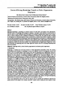
GOAL tio fri c n vel
gravity
oci ty
Figure 1: Friction Mountain Car which we describe next, each task is uniquely determined by just two parameters – the mean and variance of a friction coefficent random variable.
2.1 Friction Mountain Car To illustrate this framework, we consider an extension of the Mountain Car problem, a standard illustration used for reinforcement learning. In the original problem, a car begins in a valley and must drive to the top of the hill on the right as quickly as possible (see figure 1). The speed of the car when it reaches the goal does not matter, only the time it takes to get there. The car can accelerate forward or backwards (right and left in the figure), or just coast. The car’s engine is not strong enough to drive straight up the right hill, so it typically has to back up part way on the left hill and then accelerate forward to gain enough momentum to get up the right hill. In fact, depending on the strength of the engine, the car may have to go back and forth several times before building up enough speed to reach the top. The rewards are -1 on every time step (no discounting) until the car reaches the goal, which ends the task. We add a friction term to the physics of the mountain car. For simplicity, we model sliding friction. Every single task Ti has an associated friction coefficient distribution Fi . On each time step an instantaneous friction coefficient is drawn, independent of state and friction history, to determine the deceleration of the car due to friction during the time step. A friction distribution Fi with low mean might represent a task where the road is clear, and an Fi with high mean a case where 4
the road is rough or there is debris. A friction distribution, along with the standard parameters of the Mountain Car problem, fully specifies the transition probabilities of a Friction Mountain Car task. Though it is not required by our algorithms, in our experiments we always use a uniform distribution PT over tasks. Thus, when we specify a set fFig of friction distributions, we implicitly define an entire task distribution for the Friction Mountain Car.
3 Algorithms We use the options framework to describe temporally abstract actions (Sutton, Precup & Singh, 1998). An option consists of a policy � : S � A 7! [0; 1℄, a termination condition : S 7! [0; 1℄, and an initiation set I � S . Given an MDP and set of options O , the optimal option-value function Q�O is given by:
n
o
� (s0 ; o0 ) E (o; s) ; Q�O (s; o) = E r + k max Q O o 2O 0
(1)
where E (o; s) denotes the event of o being initiated in s, r is the total discounted reward received during the execution of o, is the discount factor for future rewards, k is the time at which the option terminates, and s0 is the termination state of the option. If the agent can compute the correct Q�O , then it can just pick options greedily according to this value function, and its behavior in the given MDP would be optimal with respect to that set of options. We use two different algorithms for computing option-value functions that can be used for behaving, given our problem definition. The Average Value Function (AVF) algorithm is the simpler one and it requires virtually no prior knowledge. AVF completely ignores the fact that multiple tasks are being solved and keeps a single state-option value function Q over the state space. We use standard SMDP Q-learning backups (Bradtke & Duff, 1995; Parr, 1998) to learn the value function. If the agent observes state s, chooses option o, and as a result ends up in state s0 and receives return r along the way, the value of the state-option pair (s; o) is updated by:
Q(s; o)
Q(s; o) + �(r + k max Q(s0 ; o0 ) Q(s; o)) o 0
(2)
where � is the learning rate. In general, there is no theoretical guarantee for the performance of the AVF algorithm. In the worst case, for instance, we can imagine a pair of linear MDPs 5
with diametrically opposed rewards. AVF would learn a value function with no useful information. Of course, in this case no value function transfer is possible. Our second algorithm is nearer the other end of the spectrum in terms of prior knowledge required and theoretical guarantees. We have noted that our task distribution model can also be thought of as a POMDP, where the state of the task is observed but not the identity of the task itself. Although solving POMDPs is very difficult, we incorporate ideas from POMDP theory in our algorithm. In particular, the agent keeps beliefs about the state it is in and uses these in its action selection. The Separate Value Functions algorithm (SVF) maintains an option-value function Qi for each task Ti ; i = 1 : : : n. The agent also maintains a set of beliefs about which task it is currently executing. Let Bi be the belief of the agent that it is solving task Ti 2 T . On starting a trial, the beliefs are initialized to the distribution over the tasks PT for all i:
Bi = PT (Ti )
After each action, the transition to the new observed state gives the agent information about which task it is in, and the belief about being in each task is updated according to the probability of the observed transition in the task. Updating is done in the standard Bayesian way. Specifically, on seeing the transition from state s to s0 by action a, the beliefs change by:
pi;a s;s Bi ; Pn j;a j =1 ps;s Bj
Bi
0
(3)
0
where pi;a s;s is the probability of the observed transition in task Ti . For temporally extended options the beliefs are updated by the same equation at each step while the option is running. This update rule assumes that the rewards do not convey specific information regarding the current task. If the rewards come from a discrete distribution that is different for each task, they can be accounted for in the same way in which we account for the transition probabilities. If the agent is in state s and has a set of beliefs Bj ; j = 1 : : : n, it assigns value to its options by computing a belief-weighted average of the option values for each task. In other words, the option it considers best to choose given s and the beliefs Bj solves the problem: 0
arg max o
n X j
=1 6
Bj Qj (s; o)
The SVF algorithm incrementally learns the value functions for each of the separate tasks. Each time an option is executed, SVF updates the action values for every task, whether the agent is actually in that task or not. To do so, it uses the SMDP Q-Learning backup, where now the Q(s; o) are replaced by the Qj (s; o) specific for the task. However, the learning rate � is additionally multiplied by the posterior belief that the agent is in the task j – i.e. Bj after the option has finished. This correction accounts for the fact that Q-values are being updated even when the agent is solving a different task. All the value functions Qj converge with probability 1 to the correct Q-values, Q�j for each task, under the assumption that the value function is represented in tabular form, and each state-action pair is experienced infinitely often in each task. Proof: Under these assumptions, the convergence proof is an application of Theorem 1 from Jaakola, Jordan & Singh (1994). The only interesting part of the proof is showing that the update operator yields a contraction. The main idea is that we are allowing the learning rate to vary with time, according to the beliefs Bi . The beliefs Bi also account for the difference between the sampling distribution for the next state s0 and the distribution of s0 in task i. For simplicity, we present here the case of primitive actions (the case of temporally extended options is similar). Let us denote by Bi;t the agent’s belief that it is in task i at time t during the trajectory (i.e. before seeing the transition from st to st+1 under action at . It is straightforward to show by induction that for any trajectory experienced by the system, the current belief for that trajectory is:
p Bi = P i;t ; j pj;t where
pi;t = P rfig
1
tY t0
=0
pi;a s s
t0 t0 t0
+1
We can re-write the update rule for Qi as follows:
Qi (st ; at )
Qi (st ; at ) + �Bi;t+1 (rsa + max Qi (st+1 ; a) Qi (st ; at )) a Qi (st ; at )(1 �) + �(1 Bi;t+1 )Qi (st ; at ) �Bi;t+1 (rsa + max Qi (st+1 ; a)) a t t
= +
t t
We have to show that the expected value of the update operator: (1
Bi;t+1 )Qi (st ; at ) + Bi;t+1 (rsa
t t
7
+
max Qi (st+1 ; a)) a
yields a contraction in the max norm. By subtracting the optimal value function Q�i (st ; at ), we obtain: (1
Bi;t+1 )(Qi (st ; at ) Q�i (st ; at )) + Bi;t+1(rsa
t t
max Qi (st+1 ; a) Q�i (st ; at )) a
+
Note first that if the belief of being in task i is 0, then the agent will not update the value function for task i at all. If the agent has perfectly identified a task, then the update becomes identical to a Q-learning update for that task. Therefore, we are only concerned here with the case in which the coefficients of both terms are between 0 and 1. The first term does not contribute to the decrease in the error, it just maintains the previous value function, to the extent that the agent does not believe that it is in the given task. Therefore, is suffices to show that the second term yields a contraction. P t � 0 0 For the second term, we can re-write Q�i (st ; at ) = rsatt + s pi;a st ;s maxa Qi (s ; a ). Therefore, the second term becomes: 0
X
Bi;t+1 (max Qi (st+1 ; a) a
pi;a s ;s t
t
s0
0
max a0
0
0
Q�i (s0 ; a0 ))
When taking the expected value over all possible partial trajectories � and over all tasks k , we obtain: X p
E f P i;t+1 (max pi;a Q�i (s0 ; a))g = Q i (st+1 ; a) s ;s max a a p j j;t+1 s X XX pi;t+1 pi;a (max Qi (st+1 ; a)
P rfkgP rf� jkg P s ;s a j pj;t+1 � k s X X
pi;t+1 (max Q Q�i (s0 ; a)) = pi;a i (st+1 ; a) s ;s max a a t
t
0
0
t
0
t
�
X
�t
X
�t
X
�t
�
pi;t
X
st+1
st+1
pi;t (
X
�t
X
st+1
pi;t
t
pi;a Qi (st+1 ; a) s ;s +1 (max a
X
pi;t (
s
0
t
t
p
t
i;at st ;st+1 (max a
p
i;at st ;st+1 (max a
X
st+1
p
i;at st ;st+1
Qi (st+1 ; a) Qi (st+1 ; a)
max a
t
0
max a
Q�i (s0 ; a)) =
0
X
s
pi;a s ;s t
t
0
((
X
st+1
X
s0
p
max
0
a0
Q�i (s0 ; a0 )) =
pi;a s ;s +1 ) t
t
i;at st ;s0
t
max a0
X
s
0
pi;a s ;s t
t
0
max a0
Q�i (s0 ; a0 ))
Q�i (s0 ; a0 )) �
jQi(st+1 ; a) Q�i (st+1 ; a)j � jQi(st+1 ; a) Q�i (st+1 ; a)j
q.e.d The SVF algorithm offers the strong guarantee of convergence to correct option values for individual tasks. In task distributions where a small number of 8
transitions quickly identifies which task the agent is solving, we can hope for performance near the optimal POMDP behavior. However, SVF also makes strong assumptions. The agent must know the transition probabilities for all of the MDPs, as well as the task distribution PT . By contrast, AVF has very weak assumptions, so it can potentially be useful in a broader range of applications.
4 Experiment Details In order to study the empirical properties of the AVF and SVF algorithms, as well as the merit of options for facilitating transfer, we performed several experiments on different Friction Mountain-Car task distributions. Here we complete the description of the environments we use, and give details on the learning methodology and performance metrics.
4.1 Friction Mountain Car Task Distributions The shape of the valley the car is trying to escape from is given by sin(3 � p) where p 2 [ �=2; 0:5℄ is the position of the car. The car’s tangential velocity v is limited to the range [ 0:07; +0:07℄. The primitive actions are three tangential accelerations a 2 f 1:0; 0:0; 1:0g. In friction mountain car we also have an instantaneous friction term f (t) drawn independently from the task’s friction distribution. The dynamics of the system is given by:
v (t + 1)
= +
p(t + 1)
=
v (t) + 0:001a 0:0025 os(3p(t)) sign(v (t)) � j0:0025sin(3p(t))f (t)j p(t) + v (t + 1)
If the deceleration due to friction exceeds the other terms, the velocity v (t+1) = 0. Both the position and the velocity are clipped to the ranges mentioned above. Additionally, if the car “hits” the lower end of the position range, its tangential velocity is set to zero. In this paper we use clipped, discretized normal distributions for the friction coefficients. The friction coefficient is allowed to take on values from 0.0 to 0.6 in increments of 0.0005. For a given mean � and standard deviation � we evaluate the corresponding Gaussian density function at each discretization point, and then scale the probabilities to ensure they sum to one. In our experiments, we consider two task distributions. Each contains 50 tasks, with friction distributions having means running in equal intervals from � = 0:2 9
to � = 0:396. The task gets increasingly difficult as friction increases towards 0.4; in fact, if f (t) = 0:4 always, the task is not solvable from some states – the car cannot even start moving. The task distributions differ only by the standard deviation of their friction distributions. We call the task distributions T0.2 and T0.02 indicating sets of friction distributions with standard deviations 0.2 and 0.02 respectively.
4.2 Options Our experiments use three main sets of options, which we call 1-Step, 20-Step and 100-Step. The 1-Step options are just the primitive actions of accelerating forward or backward and coasting. The 20-Step set also contains three options, one that accelerates forward for 20 time steps in a row before terminating, one accelerating backwards for 20 time steps, and one coasting for 20 time steps. The three options of the 100-Step set are defined similarly. At one point we compare some of those options sets with a single option which we call the Pumping option. The option, once started, does not stop until the car reaches the goal. When the car is moving backwards, the option continues to accelerate backwards until the velocity falls to zero or reverses to moving forward – i.e. until the car hits the left wall or has reached the highest it can on the left hill. Then the pumping option accelerates forward until the goal is reached or velocity flips again. The option does the utmost to keep pumping the car up higher on the opposing hills. If a particular task can be solved at all, then the Pumping option will find a solution, but not necessarily in the most efficient manner.
4.3 Learning Methodology The previous section defined the algorithms used in this study. The learning algorithms all used trial-based learning. In each trial, the car’s initial position and velocity are chosen uniformly randomly from the state space. The agent chooses its most preferred option 99% of the time and a random option 1% of the time. The trial ends when the car reaches the goal, and is also stopped early if 3000 pass without the car reaching the goal. For the Friction Mountain Car, the laws of physics plus the instantaneous friction coefficient uniquely determine the next state. In many cases, an agent observing a transition could reason backwards, using the laws of physics, to deduce the instantaneous friction that caused the transition. We make the simplification that the agent observes the friction coefficient directly, allowing us to express the 10
belief update diretly in terms of the friction distributions. The rewards give no information that helps identify the task. Let task Ti have friction distribution Fi , and suppose the agent experiences a sequence of state transitions as a result of instantaneous friction coefficients f1 ; f2 ; : : : ; fk . The belief update can be expressed as:
Bi
Q
Bi kl=1 Fi (fl ) Pn Qk j =1 Bj l=1 Fj (fl )
Since the state of the system is described by two continuous variables (position and velocity), we have to use a function approximator to represent the optionvalue function. We use a sparse coarse coding technique, CMAC(Albus, 1981), which discretizes the state space, using several grids with random offsets. We use ten tilings, each having ten position and ten velocity bins. Tilings have small random offsets, and the approximator is initialized to return a value of -100 for any input. This setting is considered standard for this task. Each option-value function is represented by a separate CMAC. The SVF algorithm, which keeps a separate value function for each task, simply uses an array of such CMACs; there is no generalization across tasks due to the function approximator, but only as a result of the learning rule and action selection rule.
4.4 Performance Measures Both transient and asymptotic measures of performance are of interest. We report on-line time per trial as learning progresses. Since trial times during learning reflect the random starts and the 1% exploration rate, we also report two off-line performance metrics. In off-line performance, the action with the highest value according to the value function is always selected and there is no learning. Off-line average time per trial is taken over all tasks and random starting points within each task. Offline bottom time is the time per trial, averaged over the tasks, when the car starts at rest at the bottom of the hill. This is the most difficult starting position, and hence constitutes a worst-case performance measure for the task distribution. In all the experiments, we optimized the learning rate constant parameter � for each set of options and each learning algorithm. The results reported below are for the best parameter settings in each case.
11
3000
2500
2000
Time to goal during 1500 learning, averaged over 30 1000 runs
100-step
1-step 500
20-step 0
0
10
20
30
40
50
60
70
80
90
100
Trials
Figure 2: Online time per trial for the AVF algorithm during the first 100 trials, for different sets of options, with optimized learning rate for each set 3000
2500
Time to goal 2000 during learning averaged over 30 1500 runs
100-step
1000
20-step
500
0
1-step
0
100
200
300
400
500
600
700
800
900
1000
Trials
Figure 3: Online time per trial for the AVF algorithm, for different sets of options, with optimized learning rate for each set
5 Experiments In our first set of experiments we compare the option sets 1-Step, 20-Step and 100-Step under the Average Value Function algorithm on task distribution T0.02. 12
3000
2500
Time 2000 to goal from random starts, 1500 using greedy policy, 1000 averaged over 30 runs 500
100-step
20-step 0
0
100
200
300
1-step
400
500
600
700
800
900
1000
Trials
Figure 4: Time per trial for the AVF algorithm computed offline every 50 trials, for a random sample of tasks and starting states, for different sets of options 3000
100-step Time 2500 to goal from bottom 2000 of the hill, using greedy 1500 policy, averaged over 30 1000 runs
1-step
20-step
500
0
0
100
200
300
400
500
600
700
800
900
1000
Trials
Figure 5: Time per trial for the AVF algorithm starting at the bottom of the hill at rest, averaged over all the tasks, for different sets of options Figure 2 shows the time for each learning trial averaged over 30 independent runs. As expected, longer options provide better early performance. The 100-Step option set, though beginning quite well, unfortunately fails to improve very much
13
during learning. 1-Step and 20-Step quickly surpass 100-Step, and after only fifty trials are performing almost as well as they do asymptotically. Note that this is after an average of only one training trial per task in the T0.02 distribution. Figure 3 displays the on-line average reward over a longer period of time. Learning for each of the option sets seems to have settled down to asymptotic behavior after approximately 400 trials. Figure 4 shows the off-line performance with the option sets over the same time period, sampled every 50 trials. Because of increased sample sizes, the curves are smoother than in the previous graph, but they track the means of the on-line performance curves quite well. Off-line performance is a better measure of what the car has learned to do to date. Since the off-line and on-line curves match well, the agent is behaving close to its greedy performance during learning. This simplifies tracking the learning because it means we do not really need to take time out for performance evaluation; rather, we can be satisfied simply to record the on-line results. The average time from the bottom of the valley measures the success of learning in the hardest area of the state space. Figure 5 shows this time, averaged over runs and a sample of tasks in the distribution, as learning progresses. Under the 100-Step options, the car never reaches the goal from the bottom of the valley – it always times out. 1-Step is solving some of the easy tasks, while 20-Step is solving all but a few of the hardest tasks. These results are also supported by the cumulative time to goal measured over 5000 trials for all sets of options, averaged over the 30 runs. 20-Step options average 0:0455 � 107 steps, compared to 0:0929 � 107 for 1-Step options and 0:4326 � 107 for 100-Step options. the differences between these numbers are statistically significant at the 0.05 level. Over all these graphs, the 20-step options seem not only to help the speed of learning, but also asymptote at a better performance and have lower variance in performance during learning. Theoretical results show that the primitive actions should always do at least as well on any single MDP when the value function is represented by a lookup table(Precup, Sutton & Singh, 1998). In our case, we are dealing with multiple MDPs as well as function approximation, so it is not clear what to expect. One particular difficulty with the 1-Step options is that differences in option values are small, making it hard to extract a good policy. 20Step options lead to larger differences in option values, making the value function easier to learn. This aspect of temporally extended actions may be important for practical purposes. We have mentioned that as the mean of the friction distribution approaches 14
140
130
120
Time to goal from 110 random starts 100 using greedy policy 90
Pumping option
80
20-step options 70
60
0
5
10
15
20
25
30
35
40
45
50
Task Number
Figure 6: Comparison of the time to goal from random starts for the Pumping option and the 20-step options, for every task 3000
2500
20-step options Time 2000 to goal from rest at 1500 bottom of the hill 1000
500
Pumping option 0
0
5
10
15
20
25
30
35
40
45
50
Task Number
Figure 7: Time to goal from bottom 0.4, the task gets increasingly difficult. For any value less than 0.4, however, the Pumping option can reach the goal, even from the bottom of the hill. In figure 6 we plot the expected times to goal for the best AVF configuration (20-Step, 5000 trials of learning) and for the Pumping option, for each of the 50 tasks. The horizontal axis shows tasks with friction distribution of increasing mean and standard 15
deviation 0.02. AVF is more efficient on most of the tasks and of equivalent value on the harder tasks. In starting from the bottom of the hill (Figure 7), though, AVF fails completely on the hardest tasks. The Pumping option, as mentioned before, solves any task that is solvable in principle. This shows that one option set can win on one of the metrics but lose on another, or may be good on a particular subset of the task distribution, but not as good overall. 1000
900
800
Time to goal 700 using greedy 600 policy from 500 random starts 400
1-step trained on task 49
300
20-step trained on task 49
200
1-step AVF 100
0
20-step AVF 0
5
10
15
20
25
30
35
40
45
Task number
Figure 8: Comparison of AVF and learning on the hardest task only, for different sets of options Figure 8 analyses transfer in a somewhat different way. Having noted that learning is very difficult on the high mean tasks, we compared AVF solutions learned across a whole task distribution with an SMDP Q-Learning solution trained only on the hardest task for an equal number of trials. The figure compares the off-line performance from random starts of these two algorithms with 1-Step and 20-Step options. The winner by far on solving the hard tasks is AVF with 20-Step options. The experience in solving easier tasks in the set allowed it to perform better on the hardest task than direct Q-Learning with 20-Step options on that task. The training procedure in this case is akin to shaping, in which a learning agent is presented with a sequence of increasingly difficult tasks, with the aim of getting it to perform well on a hard task. Surprisingly, the Q-Learning 20-step line is quite close to AVF 20 for the first three-fifths of the tasks, indicating considerable transfer from the hardest task 16
back to the easier tasks. Also important is the relationships of the AVF 1-step and AVF 20-step lines. The AVF 1-step performs not too much worse than AVF 20step on the easy tasks, but almost three times as badly on the hardest tasks. One interpretation is that the 20-Step set of options transfers knowledge between the tasks better than 1-Step options. Finally, although the 1-step options do transfer knowledge from the hard task to the easiest tasks as well, their performance is much worse than the other cases. Figures 9 and 10 study the transfer of knowledge from a single task to the whole set in greater detail. In each case, a value function was learned by SMDP Q-learning on a single task, and then the performance of the greedy policy with respect to that value function was tested from random starts on the whole set of tasks. In each case there were 5000 training trials. In figure 9, we observe that 1-Step and 20-Step options allow an equally good solution to the task trained on. However, the 1-Step policy’s performance degrades for the more difficult tasks, whereas the 20-Step policy is more robust. This may be because 20-Step options changes the visitation distribution over the state space, and encourages learning in areas that 1-Step options on the easiest task ignore. It may also be that the optimal 20-Step policies are more similar across tasks than the optimal 1-Step policies. Training on a middling difficult task shows a similar result 10. Performance on task 29, the target of learning, was somewhat worse for 1-Step than 20-Step and the performance across tasks of the former notably worse than under 20-Step. Finally, we turn our attention to the SVF algorithm. Figure 11 shows the performance of SVF with different sets of options. Performance shows the same general relationship and trends as in the case of the AVF algorithm, with the 20-step options being the best in terms of both learning speed and asymptotic behavior. The 20-Step options remain significantly faster that 1-Step options according to the cumulative time to goal metric. Of interest is how the performance of SVF changes on task distributions with low or high variance in the friction distribution. Low variance means tasks can be identified quickly, and hence a value function specific for that task guides behavior. However, during the learning process, rapid identifiability means that many tasks will receive very little updating and learning is expected to be slower. Figures 12 and 13 show the performance of AVF and SVF with 20-Step on task distributions T0.02 and T0.2 respectively. In the lower identifiability case, T0.2, SVF’s learning is more rapid because many different value functions are updated as a result of a single experience. Note also, however, that SVF’s performance is never faster than AVF, in any of these cases. This result is also supported by 17
1000 900 800 700
Average Time to 600 Goal from Random 500 Starts
1-step
400 300 200
20-step
100 0 0
5
10
15
20
25
30
35
40
45
Tasks
Figure 9: Performance from random starts across tasks of SMDP Q-Learned policy for task 0.
1000 900 800 700
Average Time to 600 Goal from Random 500 Starts 400
1-step
300 200 100 0 0
20-step 5
10
15
20
25
30
35
40
45
Tasks
Figure 10: Performance from random starts across tasks of SMDP Q-learned policy for task 29. the cumulative time to goal for SVF and AVF. For 20-Step options, in the T0.02 task distribution, SVF’s cumulative time to goal is 0:1803 � 107 steps, compared 18
3000
2500
1-step
2000
Time to goal during 1500 learning averaged over 30 runs 1000
100-step
500
20-step 0
0
500
1000
1500
2000
2500
3000
3500
4000
4500
5000
Trials
Figure 11: Online time per trial for the SVF algorithm, for different sets of options, with optimized learning rate for each set to 0:0455 � 107 for AVF with the same set of options. In the T0.2 distribution, the results are 0:1439 � 107 steps, vs. 0:0429 � 107 steps. These learning speed relationships are similar for the other sets of options. In terms of asymptotic behavior, the specificity of SVF is of little help with the 20-Step option set. With the 1-Step option set, we did observe SVF eventually overtaking AVF, particularly on the time-to-goal from the bottom of the valley metric. Thus, especially in the hard cases, being able to identify the task and use a specific value function does improve behavior.
6 Conclusion We have introduced a framework for studying knowledge transfer in reinforcement learning in which the learning agent has to solve different tasks drawn from a given distribution. This model allows us to compare transfer properties for different options and learning algorithms. We believe that our task-distribution model of an agent’s environment is realistic. Rarely is one asked to resolve the exact same problem one has solved before, but repeatedly having to solve very similar tasks is commonplace. Further, the tasks we need to solve as people usually have a limited time span, so considering only episodic tasks does not seem overly restrictive. 19
3000
2500
2000
Time to goal during 1500 learning, averaged over 30 1000 runs
SVF, 20-step AVF, 20-step
500
0
0
500
1000
1500
2000
2500
3000
3500
4000
4500
5000
Trials
Figure 12: Comparison of the AVF and SVF algorithms with 20-step options on the T0.02 task distribution (tasks are easy to identify) 3000
2500
2000
Time to goal during 1500 learning, averaged over 30 1000 runs
SVF, 20-step
AVF, 20-step 500
0
0
500
1000
1500
2000
2500
3000
3500
4000
4500
5000
Trials
Figure 13: Comparison of the AVF and SVF algorithms with 20-step options on the T0.2 task distribution (tasks are hard to identify) We introduced two learning algorithms, AVF and SVF, which are very different in their assumptions and properties. AVF assumes no prior knowledge and learns a single value function for all the tasks. SVF has very strong prior knowledge assumptions, but is guaranteed to converge to correct value functions for 20
each task. In our experiments we found AVF to be more effective on most of the performance measures. However, more experimentation in different domains would be needed to ascertain its practical value. Our experiments illustrated knowledge transfer between tasks under a variety of circumstances. In particular, training on a distribution of hard and easy tasks yielded better performance than training specifically to solve hard tasks. Finally, we compared different sets of options in terms of their ability to transfer knowledge. We found that temporally extended options can help in this respect (which is an expected result). Also, different sets of options exhibit different tradeoffs in terms of computation speed vs. the quality of their asymptotic behavior. We are currently working on algorithms that require less prior knowledge, while still providing theoretical guarantees. More restrictive definitions of the task distributions could also allow the development of specific algorithms with little or no prior knowledge. Another future direction for this work is in the automated discovery of options. Although options allow us, as the agent’s designer, to incorporate prior knowledge, we may also want the agent to discover options for itself. Measures of transfer are important criteria for agents trying to develop their own set of options. Although we did not study algorithms for option acquisition here, our experiments compare different sets of options with regard to their transferability. Such comparisons may be an important part of option discovery algorithms.
References Albus, J. S. (1981). Brain, behaviour and robotics, chapter 6. Byte Books. Bernstein, D. S. (1999). Reusing old policies to accelerate learning on new mdps. Technical Report TR 99-26, University of Massachusetts, Amherst, MA. Bradtke, S. J. & Duff, M. O. (1995). Reinforcement learning methods for continuous-time Markov decision problems. In Advances in Neural Information Processing Systems 7 (pp. 393–400). MIT Press. Dayan, P. & Hinton, G. E. (1993). Feudal reinforcement learning. In Advances in Neural Information Processing Systems 5 (pp. 271–278). Morgan Kaufmann. Dietterich, T. G. (1998). The MAXQ method for hierarchical reinforcement learning. In Proceedings of the Fifteenth International Conference on Machine Learning. Morgan Kaufmann. 21
Drummond, C. (1998). Composing functions to speed up reinforcement learning in a changing world. In Machine Learning: ECML98. 10th European Conference on Machine Learning, Chemnitz, Germany, April 1998. Proceedings (pp. 370–381). Springer. Hauskrecht, M., Meuleau, N., Boutilier, C., Kaelbling, L. P. & Dean, T. (1998). Hierarchical solution fo markov decision processes using macro-actions. In Proceedings of the Fourteenth International Conference on Uncertainty In Artificial Intelligence. Jaakkola, T., Jordan, M. & Singh, S. (1994). On the convergence of stochastic iterative dynamic programming algorithms. Neural Computation, 6(6), 1185–1201. Kaelbling, L. P. (1993a). Hierarchical learning in stochastic domains: Preliminary results. In Proceedings of the Tenth International Conference on Machine Learning (pp. 167–173). Morgan Kaufmann. Kaelbling, L. P. (1993b). Learning to achieve goals. In Proceedings of the Thidteenth International Joint Conference on Artificial Intelligence (pp. 1094– 1098). Morgan Kaufmann. Kalmar, Z. & Szepeszvari, C. (1999). An evaluation criterion for macro learning and some results. Technical Report TR 99-01, Mindmaker Ltd., Budapest, Hungary. Lin, L.-J. (1993). Reinforcement Learning for Robots Using Neural Networks. PhD thesis, Carnegie Mellon University. Mahadevan, S., Marchallek, N., Das, T. K. & Gosavi, A. (1997). Selfimproving factory simulation using continuous-time average-reward reinforcement learning. In Proceedings of the Fourteenth International Conference on Machine Learning (pp. 202–210). Morgan Kaufmann. McGovern, A., Sutton, R. S. & Fagg, A. H. (1997). Roles of macro-actions in accelerating reinforcement learning. In Grace Hopper Celebration of Women in Computing (pp. 13–17). Moore, A. W., Baird, L. & Kaelbling, L. (1998). Multi-value functions: Efficient automatic hierarchies for multiple-goals mdps. In NIPS’98 Workshop on Abstraction and Hierarchy in Reinforcement Learning. 22
Parr, R. (1998). Hierarchical Control and learning for Markov decision processes. PhD thesis, University of California at Berkeley. Parr, R. & Russell, S. (1998). Reinforcement learning with hierarchies of machines. In Advances in Neural Information Processing Systems 10. MIT Press. Precup, D. & Sutton, R. S. (1998). Multi-time models for temporally abstract planning. In Advances in Neural Information Processing Systems 10. MIT Press. Precup, D., Sutton, R. S. & Singh, S. (1998). Theoretical results on reinforcement learning with temporally abstract options. In Nedellec, C. & Rouveirol, C. (Eds.), Machine Learning: ECML98. 10th European Conference on Machine Learning, Chemnitz, Germany, April 1998. Proceedings, Volume 1398 of Lecture Notes in Artificial Intelligence (pp. 382–393). Springer. Singh, S. P. (1992a). Reinforcement learning with a hierarchy of abstract models. In Proceedings of the Tenth National Conference on Artificial Intelligence (pp. 202–207). MIT/AAAI Press. Singh, S. P. (1992b). Scaling reinforcement learning by learning variable temporal resolution models. In Proceedings of the Ninth International Conference on Machine Learning (pp. 406–415). Morgan Kaufmann. Sutton, R. S. (1995). TD models: Modeling the world as a mixture of time scales. In Proceedings of the Twelfth International Conference on Machine Learning (pp. 531–539). Morgan Kaufmann. Sutton, R. S., Precup, D. & Singh, S. (1998). Between MDPs and Semi-MDPs: learning, planning, and representing knowledge at multiple temporal scales. Technical Report 98-74, University of Massachusetts, Amherst, MA 01003. Thrun, S. & Schwartz, A. (1995). Finding structure in reinforcement learning. In Advances in Neural Information Processing Systems 7 (pp. 385–392). MIT Press.
23