Using Performance Incentives to Reward the Value Added by Educators

Using Performance Incentives to Reward the Value Added by Educators: Theory and Evidence from China Weili Ding Steven F. Lehrer University of Pittsburgh University of Pittsburgh January 31, 2000 Abstract

Over the last thirty years, education reform has been a active topic of debate among policy makers and social scientists. The majority of proposals for reform have been based on a combination of regulations and fixed definitions of school - the resources, organization and structure of schools and classrooms. However, recently increased attention has been directed to the results of the school. Reform proposals have suggested policies that are built on what students actually accomplish and reward instructors who induce good performance by students. In this paper we demonstrate that incentive contracts based on a combination of objective and subjective performance evaluations can mitigate incentive distortions caused by imperfect objective measures. Moreover, when we combine the explicit contract based on an objective performance measure with the implicit contract based on a subjective performance measure, the combined incentive provided (supported by trigger strategy) are increasing with the variation of the objective performance measure. We then test the performance of our model using data from China. In China, administrators evaluate the performance of teachers and this evaluation is used to determine a component of teacher compensation. Our estimates indicate that teacher salaries are indeed positively related to objective performance and subjective performance measures. We find that increases in salary are greater for higher ranked instructors. Finally, we find that although education and sex do not affect salary they are significantly related to the probability of promotion. Instructors who are more educated, married, male, experienced and who encounter fewer students within a week are more likely to be higher ranked.

We are grateful to Thomas Rawski for much support and numerous discussions which have encouraged us to complete this study. We wish to thank John Engberg, Esther Gal-Or and Jean Francois Richard for comments and suggestions which have helped to improve this paper. We also wish to thank the University of Pittsburgh China Council for research support. The usual caveat applies. 1

1

Introduction

A common thread runs through many recent proposals for the reform of American K-12 education system: the notion of using students’ performance on achievement tests or assessments as a basis for rewarding educators and school systems. The logic behind these proposals is simple and compelling: since student achievement is the primary goal of education then providing teachers with incentives tied to the amount of learning they induce would focus and intensify their efforts. The proposal of the Panel on the Economics of Education Reform (PEER) (Hanushek et al. 1994) is an example of a reform approach that would rely heavily on holding educators accountable for improving student’s performance. The PEER proposal focuses on three elements: the efficient use of resources, continuous adaptation and performance incentives for educators based on assessments of student performance. The proposal asserts that effective management requires a system take into account the many sources of educational performance, some of which are not the responsibility of the school, and maintains that schools should be held accountable only for their value added. In the United States teacher compensation has typically been tied to extrinsic measures of quality, such as highest degree attained. However, the many studies that have examined the relationship between such extrinsic measures and student performance find little correlation1. The lack of a relationship between resources and performance surprises many people but perhaps should not. Schools are easily distinguished from other more successful institutions in that rewards to their employees are only vaguely associated with performance. A teacher who produces exceptionally large gains in her students performance generally sees little difference in compensation, career advancement or job status when compared with a teacher who produces exceptionally small gains. With few incentives to obtain improved performance, it should not be surprising that resources have not been systematically used. Since it is student achievement that matters, there is a growing interest in the United States in tying the compensation of teachers to measures of their performance. One might measure a teacher’s performance by the performance of that teacher’s students, factoring out the contributions that are attributable to other influences, such as prior achievement and peer group effects. This approach presumes that whatever variations in the average of student test performance from class to class that cannot be accounted for by measured differences must be attributed to differences in the quality of instruction across classrooms. This approach is not feasible since it relies on the presumption that accurate measures of peer and family effects exist. Yet this presumption may not be warranted. There is some limited evidence that the subjective evaluation of principals and school administrators of the effectiveness of the teachers can be highly correlated with achievements of students2. If such

See Hanushek (1986) for a survey of studies that have attempted to account for teacher skill differences. Measures include indicators if the teacher is teaching the subject in which she was granted a degree, principals’ evaluations, teaching techniques and as discussed in the text the highest degree obtained. Munrane (1981) found that students taught by effective teachers learn much more in school than students who 1

2

2

subjective valuations are good predictors of student achievement then they might be used as a basis for a performance based payment system. In China, administrators and distinguished teachers evaluate the performance of teachers. This evaluation along with other factors are used to determine a significant component of teachers’ compensation. We have collected a unique data set from east China that allows us to measure the contribution of the quality of the teachers a student has had access to during the course of her secondary school education to that student’s academic achievement, as measured by scores on college admission examinations. The goal of this paper is to design a contract between the school boards and teachers which includes incentives for both objective and subjective performance to motivate and increase teachers’ effort. We then test the predictions of this contract using data from China. Performance contracts typically involve developing explicit contracts that base rewards on meeting various performance goals. There exists a great fear that such contracts could distort the behavior of educators and students. For example, tying pay to performance on specific tests may lead to narrowing of instruction within subject areas as instructors reduce their emphasis on untested subject areas. Instructors further may increase the use of in class drills and test preparation sessions. Furthermore, since there is no single agreed upon best approach to performing specific educational tasks, it is simply not possible to design policies that are based on full descriptions of what is to be done and how it is done in the classroom3. An additional complication is that there are other desired outcomes of schooling. Much of what many individuals need to learn will arise after they leave public schools in later education, in the workplace and in civic life. The extent to which they are successful in this later learning may depend in a substantial part on the body of knowledge and skills that students have at graduation, much of which can be tested. But is also likely to depend on attitudes and habits that are not typically measured by achievement tests. Thus an accountability system that produces high test scores at the price of poor performance on unmeasured outcomes may be a poor bargain4. In this paper, we demonstrate (similar to Baker, Gibbons and Murphy [1994]) that an incentive compensation scheme composed of objective and subjective performance evaluations provides the proper incentives for teachers in a world where neither output is verifiable nor teacher effort observable. The idea underlying the model is that subjective performance evaluations (i. e. principal’s evaluations) can be used to correct for any possible distortion in teacher incentives generated by an objective performance evaluation (student test scores). This paper is organized as follows. In the next section we introduce our model and demonstrate how an incentive scheme composed of objective and subjective performance evaluations can increase

are taught by ineffective teachers. There are many equally effective approaches to learning various subjects and skills, differentiated by how individual students and teachers adapt to specific tactics and techniques. See Haney and Raczek (1994) for a discussion. 3 4

3

teacher effort. In section III we describe the secondary education system in China and discuss the data that we utilize to estimate our model. This is to the best of our knowledge the first study to employ individual level data on students and school inputs from China. We empirically examine China’s salary schedule in detail in Section IV. We find that the system in China is indeed rewarding teachers based on the criteria upon which it is designed and that there are strong financial incentives for teachers to improve their performance. Our concluding thoughts and directions for future work are provided in section V. 2

Theory

2.1 The economic environment Our model extends the benchmark model discussed in Baker, Gibbons and Murphy (1994) (henceforth referred to as BGM).5 We consider a repeated game between a school and a teacher. The school board is not sure of the teaching quality of an individual at the time she hires her. There are two types of teachers existing in the job market. With probability , the school meets with a teacher of type (teacher with high teaching ability); and with probability 1

α

H − α, the teacher is of type L (low teaching ability). The school’s objective in a labor contract is to maximize the value added by each educator of its student body (hc) each period. For simplicity, we assume hc takes the value of either zero or one. Each period, the teacher chooses an unobservable effort level e, which stochastically determines her contribution to school’s objective hc. When the teacher is of type H and chooses her effort level to be e, hc equals one with probability ε : prob{hc = 1| e,H } = ε. When the teacher is of type L and chooses her effort level to be e, hc equals one with probability pε: prob{hc = 1| e,L} = pε, where e ∈ [0, 1] and p ∈ (0, 1). Thus p is the productivity difference between high and low ability teachers. We assume the teacher’s contribution to the students’ human capital is too complicated and subtle to be included in any explicit contract but otherwise can be subjectively evaluated. The teacher’s effort also contributes to a second variable t, which can be objectively evaluated. An example of t in the real world would be students’ test scores. We assume t to be either zero or one as hc. Let µ define the difference between the effect of a teacher’s effort on school’s objective hc and that on objective performance measure t. µ is private information to a teacher in each period realized before she exerts effort but after she accepts the contract. Thus the probability that t = 1 is µ · ε.6 This private information can be interpreted as the state of the students she faces in each

There are two major differences between our model and that of BGM. First, we introduce teacher’s type as hidden information. Second, teacher cannot be fired once hired by assumption while in BGM, a firm can decide to fire a worker after any period even though in equilibrium, the worker is never fired. We assume that the support of µ and the shape of the disutility function introduced later are such that µ ε < 1. 5

6

·

4

period. If the students she has are disruptive, then high effort increases to devote more effort teaching discip

hc

but not

t since she has

line and less in knowledge – µ is close to zero; if the students are well disciplined, high effort increases both hc and t – µ is close to one; if the students are well disciplined and well-equipped in test skills, small effort can increase t but not hc since students can be taught to memorize knowledge without really understand it – µ is greater than one. We assume E {µ} = 1: on average t is an unbiased measure of hc. The school can offer a contract based on a fixed salary s, a bonus β 1 paid to the teacher when t = 1 is realized and a bonus β 2 paid to the teacher when hc = 1 is realized. For simplicity and the purpose of static comparison we consider the optimal linear incentive contracts. However, in the empirical sections that follow we will restrict our attention to the institutional environment where only one contract can be offered to either type of teacher. This means that teachers cannot be differentiated by different contracts offered up-front. The timing of the events in each period is as follows: First, the school offers the contract (s,β1,β2) to the teacher. Second, the teacher decides whether to accept this contract. Her reservation payoff (utility) from an alternative employment opportunity is WH if her type is H and WL if her type is L. After she accepts the contract, she will observe the state µ and decides her effort level e. At the end of the period, hc and t are realized and the school pays the teacher s and β1 according to the contract but will decide whether to honor β2 since it’s non-verifiable by a third party. Upon receiving a contract, H type teacher decides her effort level eH such that 2 max eH s + µeH β 1 + eH β 2 − γeH

and

(IC1)

L type teacher decides her effort level eL such that max s + µpeL β 1 + peL β 2

eL

− γe2L

Solving the first order conditions, we derive the optimal effort levels

eH (µ, β 1 , β 2 )

=

eL(µ, β 1 , β 2 )

=

5

µβ 1 + β 2 , 2γ µβ 1 + β 2 p 2γ

(IC2)

2.2 The optimal contract with no incentive compensation. From the first order conditions it is easy to see that the effort level of both teacher types would be zero7 if no incentive compensation is offered. The school’s expected payoff is i depending on which type of teacher they would hire. It is obvious that the school would only want to hire a L type teacher since it costs them less. That yields the first proposition of the model

−W

Proposition 1 The optimal fixed salary contract is (s = WL). Only the low ability teacher would accept this contract and zero effort is exerted regardless of the realization of the state (µ).

2.3 The optimal explicit contract based on the objective performance measurement. If an explicit contract (s, β 1 ) is accepted, the high ability teacher would choose effort level eH (µ, β 1 ) = µβ 1 µβ 1 and the low ability teacher would choose effort level eL (µ, β 1 ) = p for each realization of 2γ 2γ µ. Thus high ability teacher will accept the contract if the expected utility from this contract is at least as large as her outside options:






· − γe2H ≥ WH for eH derived as above;

Eµ sH + µeH β 1

(IR1 )

and low ability teacher accepts the contract if it’s no worse than her outside options






· − γe2L ≥ WL for eL derived as above.

Eµ sL + µpeL β 1

(IR2 )

The minimum base salary for each teacher type to accept the contract would be

=








− Eµ µpeL · β1 − γe2L β2 WL − p2 [1 + var(µ)] 1 4γ

sL (β 1) = WL =




− Eµ µeH · β1 − γe2H β 21 WH − [1 + var(µ)] 4γ

sH (β 1 ) = WH

7 or some minimum effort level the school has to and can observe from its teacher in order to continue the

employment relationship with its teacher. That is under the assumption that the least able teacher can be detected by the school and be dismissed as a result.

6

When the minimum base salary for the high ability teacher is greater than the minimum base salary for the low ability teacher, the school has two choices8 :

s s β

1. Set = H ( 1 ) so that both types of teachers accept the contract. In this case the school’s expected payoff would be

V (β1)

= =

Eµ {[αeH + (1 − α)peL ] − s − αµeH β1 − (1 − α)µ · peLβ1} A β 2γ 1

1 2 − 2A4− [1 + var (µ)]β 1 − WH γ

where A

≡ [α + (1 − α)p2] ∈ (0, 1)

the optimal explicit contract derived from the first order condition is

β ∗1 = =

{} { }

− −

Eµ µ [α + (1 α)p2] Eµ µ2 [2α + 2(1 α)p2 1] 1 A [1 + var(µ)] (2A 1)

·

−

> 0 if A

−

≡ [α + (1 − α)p2] > 21

The school’s expected payoff by offering (s = sH (β ∗1 ) , β 1 = β ∗1 ) is

V That is valid if WH

(β ∗1

A2 |s = sH ) = 4γ [1 + var{µ}] · 2A − 1 1

− WH

2

2

− WL > (1 − p2)[1 + var(µ)] 4βγ1 = 4γ [1 + 1var{µ}] · (2AA− 1)2 · (1 − p2).

2. Set s = sL (β 1 ) such that only the low ability teacher would accept the contract. The school’s expected payoff is

{

V (β 1 ) = Eµ peL

− s − µ · peLβ 1}

the optimal explicit contract derived from the first order condition is 8

I f sH > sL , ie, WH

2

− WL > (1 − p2 )[1 + var(µ)] 4βγ1 , 7

(case 1)

β ∗1 =

1

2 1 + var(µ) p > 0

with school’s expected payoff to be V (β ∗1|s = sL) =

1

· p2 − WL 4γ [1 + var{µ}]

The second case is valid with only L type accepts the contract at WH − WL > 4γ [1 +1var(µ)] · (1 − p2)p4. As the variance of µ increases, t becomes a much noisier measure of hc. It’s intuitive to see the

bonus attached to the objective performance measure β ∗1 becomes smaller since the school doesn’t want to provide a distortionary incentive. The school decides to hire both type of teachers if9 1

4γ [1 + var



{µ}]

A2 2A − 1

−p

2



> WH

2

− WL > 4γ [1 + 1var{µ}] (2AA− 1)2 · (1 − p2)

(V1)

The gap between the LHS of (V1) and the RHS of (V1) becomes wider as the variation of µ decreases. This implies that (V1) is more likely to be the case if the objective performance measure is a better signal for the school’s goal. Somewhat ”controversial” is that as α increases, the school is less willing to attract high ability teacher (s =sL is more likely) since the gap becomes narrower as the fraction of high ability teachers in population increases. The intuition behind this is that the school is more likely to pay β 1 if the teacher is more likely to be of high ability, which increases the school’s wage cost if both type of teachers are attached.

base salary for a high ability teacher is higher than the minimum base salary for a low ability teacher, it’s possible for the school to offer an explicit contract to both type of teachers (V1). The bonus attached to the objective performance measure is close to zero if varµ is a very noisy assessment of the teacher’s value added. Moreover, this explicit contract yields higher value for the school than a contract with no incentive compensation. Proposition 2

If the minimum

9 (V1) comes from the relation in case 1 and the following inequality

V (β ∗1 |s = sH ) > V (β∗1 |s = sL )

8

Since the explicit contract is based on the quality of the objective performance measure, the variance of the measure decides the power of the incentive in any optimal contract, otherwise distortionary performance will be generated. When the measure is a very noisy assessment of a teacher’s real contribution, the bonus to this objective measure is close to zero and the effort level exerted by the teacher is not much higher than under a fixed salary contract. Thus, the feasibility of an explicit contract depends on the difference between the objective evaluation and the real contribution

2.4 The optimal contract based both on objective and subjective performance measurement

We first consider the simple case where the subjective performance measurement is nonverifiable but otherwise perfect. This case can be generalized to situations where the subjective performance measure is a better measure of the teacher’s contribution to her students than the objective performance measure. A contract that compensates a teacher not only on her students’ test scores, but also on some subjective performance measure like students’ evaluation, the principal’s evaluation or her colleague’s evaluation is considered to be fairer or more balanced than any explicit contract. But from the school’s perspective, such a contract would be offered only if it improves the school’s value. In this section we investigate the relationship between objective performance measure and subjective performance measure in the combined-incentive contract. If such a contract (s, β1, β2) is accepted, high ability teacher exerts effort eH = µβ12+γ β2 and low ability teacher exerts effort eL = µβ 12+γ β 2 p. Then the minimum base salary for high ability teacher is




· − γe2H ≥ WH for eH = µβ12+γ β2

·

Eµ sH + µeH β 1 + eH β 2




− Eµ µeH · β 1 + eH · β2 − γe2H [1 + var(µ)]β 21 + 2β 1 β 2 + β 22 WH − 4γ

sH (β 1 , β 2 ) = WH =

= sH (β 1 )

−

2

2β 1β 2 + β 2 4γ

9



< sH (β 1 ) for (β 2 > 0)

(III.IR1 )

and the minimum base salary for low ability teacher is




·



· − γe2L ≥ WL for eL = µβ12+γ β 2 p

Eµ sL + µpeL β 1 + peL β 2



− Eµ µpeL · β1 + peL · β2 − γe2L 2 2 2 [1 + var (µ)]β 1 + 2β 1 β 2 + β 2 WL − p 4γ

sL (β 1 , β 2) = WL =




(III IR2 )

= sL (β 1)

2

− p2 2β1β42γ+ β2

< sL (β 1 ) for (β 2 > 0)

se salary for either type of teacher to accept the contract is lower than that in a contract only reward teacher for her objective performance. Similar to the analysis in the previous section the school has two choices if sH (β1, β2) > sL(β1, β2) and setting s = sH (β1, β 2) makes it possible to hire either type of teacher. If (s = sH , β1, β2) is the enforced contract, the school’s value would be We notice that under the combined incentive contract, the required minimum ba

= Eµ {[αeH + (1 − α)peL] − s − α(µeH β1 + eH β 2) − (1 − α)(µ · peLβ 1 + peLβ 2)} = 2Aγ (β1 + β2) − 2A4γ− 1 [(1 + varµ)β 21 + 2β1β2 + β22] − WH = V (β1) + 2Aγ β2 − 2A4γ− 1 (2β 1β 2 + β22) 1 < 1 and A ∈ ( 1 , 1) > V (β 1 ) for 0 < β 2 + 2β 1 < 1 − 2A 2 2 But different from the previous section, the school can renege on the ”promised” subjective performance bonus at the end of each period since hc is not verifiable by a third party. We use the ”self-enforcement” concept here to enforce an implicit contract. That is to say, the school would not renege the contract because it’s better off for the school in equilibrium. If the school reneges at the realization of hc = 1, the savings in salary would be β2 for that period. Afterwards, the teacher would never believe that the school would deliver β2. From next µβ 1 period on, she will adjust her effort level to eH = µβ if she is a high ability teacher and eL = 1 p 2γ 2γ 10 if she is a low ability teacher . The expected value gain from paying the subjective performance V (β 1 , β 2)

10 This is actually assuming that the teacher uses trigger strategy, which is the most severe credible punishment

for the school.

10

bonus would be

V (β 1 , β 2 )

− V (β1) , where r is the school’s discount rate.

Then the school should r honor the implicit contract if and only if the expected gain of honoring the contract exceeds the savings in salary if it reneges this period: A

− V (β1) ≥ β ⇔ 2γ 2 r

V (β 1 , β 2)

β2 −

2A

− 1 β (2β

4γ

2

1

+ β 2)

r



≥ β2



A 2A − 1 2A − 1 i.e.β 2 − β1 − β2 − r ≥ 0 2γ 2γ 4γ

(V2)

The optimal contract sets β 1 and β 2 to maximize V (β 1 , β 2 ), subject to the reneging constraint (V2). Define λ as the Lagrange multiplier for (V2). The optimal contract satisfies

∂L ∂β 1

=

A 2A − 1 2A − 1 − [(1 + varµ)β 1 + β 2] + λβ 2(− )=0 2γ 2γ 2γ

(10a)

A 2A − 1 A 2A − 1 2A − 1 − (β 1 + β 2 ) + λ( − r− β1 − β 2) = 0 (10b) 2γ 2γ 2γ 2γ 2γ A When λ is zero, one of the optimal contract is to offer β 2 = and β 1 = 0. The optimal 2A − 1 contract involving both subjective measurement and objective measurement must have λ = 0, which A 2A − 1 2A − 1 A 2A − 1 2A − 1 implies − β1 − β2 − r = − + β1 + β2 + r = 0 2γ 2γ 4γ 2γ 2γ 4γ ∂L ∂β 2

=

− 10b = − 2A2γ− 1 (varµ)β 1 + λ(− 2Aγ + r + 2A2γ− 1 β1) − 2A − 1 (varµ)β + λ(− 2A − 1 β ) = 0

0 = 10a =

2γ

4γ

1

λ = −2(varµ) 11

2

β1 0 if

varµ

A > 2γr(1

1 − varµ )

11

β ∗∗ 1 =

A

(2A

− 4γr

− 1)(1 + varµ)


4γr > 0

and ∗∗ β ∗∗ 1 + β1 = 11 β

2

>0

2varµ(A − 2γr) + A · > β ∗1 2A − 1 (1 + varµ) 1

− 2varµγr + 2γr) − 4γr = 2varµ(A−4γr) − 2A4γr− 1 = 2(varµA (2 A−1)(1+varµ) (2A − 1)(1 + varµ) 2A − 1 1 if (4γr < 1) and A ∈ (max( 2 , 4γr), 1)

12

β ∗∗ + β ∗∗ 1 Under the combined incentive contract, the expected effort from either type of teacher ( 1 2γ β ∗∗ + β ∗∗ 1 for high ability teacher and 1 p for low ability teacher) is higher than that in the explicit 2γ ∗

∗

β β contract ( 1 for high ability teacher and 1 p for low ability teacher). 2γ 2γ

∗∗ We can see that β ∗∗ 1 is decreasing with varµ while β 2 is increasing with varµ. It’s natural to expect that as the objective performance measure becomes much noisier relative to the subjective performance measure, the school relies more on the subjective measure. Moreover, it’s interesting to observe that the total bonus size is larger than in any optimal explicit contract and the size actually grows with varµ, the noise. The intuition behind this is that as varµ increases, the school has to reduce the bonus size attached to the objective performance; otherwise distortionary incentive would drive the teacher to exert greater effort when there is a good chance of raising the students’ test scores (µ is large) and to shirk effort when the chance of improving students’ test scores is small. Therefore the bonus attached to subjective performance β 2 has to increase for proper provision of incentive to the teacher. However, increased β ∗∗ 2 gives the school a higher incentive to renege the implicit contract when hc = 1 is realized. Therefore the expected value gain from honoring the implicit contract (rβ 2 ) has to be greater for the school not to deviate in equilibrium. This results in higher bonus offered by school in equilibrium as varµ increases:.

∂β ∗∗ 2 ∂varµ

∂ (β ∗∗ 1

+

β ∗∗ 1 )

∂varµ

∂ =

=

A − 4γr · 2A − 1 (1 + varµ)2 2

2(varµA − 2varµγr) + A · 2A − 1 (1 + varµ)

>0

1

∂varµ

=

A − 4γr · >0 2A − 1 (1 + varµ)2 1

Proposition 3 When both subjective and objective performance measures are used to provide incentive to teachers, the feasibility of an incentive compensation scheme does NOT depend on the quality of the objective measure anymore due to the substitutability of an subjective measure. Moreover, teacher’s effort is highest in this scheme. The proof is trivial. In this section we demonstrated that an incentive compensation scheme composed of objective and subjective performance evaluations provides the proper incentives for teachers in a world where 13

neither output is verifiable nor teacher effort observable. An incentive contract based on this combination of objective and subjective performance evaluations can mitigate incentive distortions caused by an imperfect objective measure. Moreover, when we combine the explicit contract based on an objective performance measure and the implicit contract based on a subjective performance measure, the combined incentive provided (supported by trigger strategy) is increasing with the variation of the objective performance measure. In the next section we describe the data that we have collected to estimate the parameters of the wage equation.

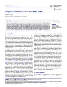
3 China’s Secondary Education System and Data To estimate the parameters of our wage contract we use a data set collected by the authors in a county in the Jiangsu province of China12. The data set is first composed of administrative records from ten of the county’s fourteen secondary schools. These records provide us with individual level information on over 1500 teachers’ demographic variables, education, salary and employment. Information on the teaching load, subjects taught and the measure of teacher quality (rank) for both 1995 and 1998 is also contained within. Before describing the contents of the data set in greater detail it is important to briefly describe the current system of secondary education in China. As in the United States, local school boards determine the curriculum in each county. The school board regulates the textbooks and minimum standard for grade promotion but gives teachers the freedom to use their own teaching method. However, the local school board assesses the quality of each individual teacher’s instruction. Based on these assessments, teachers ranking within the education system can be promoted from intern (newly hired) to third-class, to second-class, to first class and finally superior teacher. These rankings as well as years of teaching experience determine components of teachers’ salaries. In figure 1 we plot the salary scale for teachers of different ranks over the years of teaching experience using 1998 data. It is clear from this figure that teachers have a strong incentive to be ranked as a superior teacher within their first twenty years. Notice further, that irrespective of the years of experience the gap in salaries between teachers of different ranks increases as the ranking increases thus the system provides strong financial incentives for teachers to improve their ranks. It is important to note that teachers may also receive non pecuniary (psychic) income from the title once promoted. Teachers of higher rank also earn higher wages in outside employment opportunities such as tutoring. Finally, it is clear from the above diagram that the salaries follow a rule of thumb and are not determined in the manner suggested by our model. In the next section, we will discuss how we can estimate these theoretical parameters from the above salary schedule. 12 This dataset is confidential and as per our agreement with the local government we are not allowed to mention

the county by name.

14

Superior Teacher 2nd Class Teacher

1st Class Teacher 3rd Class Teacher

14000

12000

10000

8000

6000

4000 1

5

10

15 20 25 30 Teaching Experience (Years)

Figure 1: Teacher Salary Scale by Teaching Experience in 1998

15

35

In conducting assessments and determining whether an instructor will be promoted the school board examines five factors. First, they examine teaching skills. They examine the performance of that teacher’s students relative to other instructors on entrance examinations and other assessments. Administrators and instructors within the same school in that subject area randomly attend the candidate’s lectures to evaluate the quality of instruction. Furthermore, credit is given to teachers who introduce new effective teaching methods in the classroom. Second, the quality of the school and years of education that the instructor had completed are assessed. A national five point ranking system of higher education institutions is used to assess the quality of colleges and universities the teacher got her degree in. This information is combined with the number of articles the instructor had published on instructional methods in teaching journals to get a measure of teacher’s knowledge. Thus, this system provides a strong incentive for teachers to introduce new teaching methods and if they are effective an article describing the method and evaluating the results can be published in a teaching journal. Third, a teacher’s ability to regularly evaluate and monitor the performance of her students, detect problems that affect her students (intellectually or socially) and the efficacy in which these problems are dealt with are evaluated. Fourth, whether a teacher is enthusiastic while performing her job and concerns for her students performance (e.g. promptness in getting in touch with the students’ families) is also assessed. Finally, the teacher’s work ethic is monitored. School board officials argued that incentives to be higher ranked have increased recently as the difference in salaries across teachers of different ranks for a given level of teaching experience has widened. Teachers salaries are increased in China through the finances of each local government, which reflects the willingness of the society to reward its teachers. Local Chinese government usually associates its economic growth with the increased education level of its population in their annual report and even advertises the number of superior teachers in its schooling system to attract outside investment. The officials also pointed out that the nationwide introduction of this system in the early 1980s increased not average effort exerted by the teachers but more so average concern towards students. Instructors would more closely monitor student performance and contact the family either by phone or by visit when a child encountered difficulties. As well, instructors increasingly tutor students who are falling behind and form peer groups of students to tutor students who are falling behind. These actions directly increase subjective evaluations and indirectly increase objective performance evaluations. Not only are the teachers ranked but there is a clear ranking of the quality of instruction at each school within a county. It is common knowledge among the population whether a school is considered to be either a national model school or a provincial model school or a school that focuses on teaching students trade skills. Students compete for positions in the higher quality schools by writing a municipal level high school entrance examination at the completion of junior high school13. 13 The definition of a municipality in China differs markedly from that used in North America. In China, there are

16

This exam covers material in six subject areas and is held over a period of three days14. Scores on this exam are almost the sole determinant of high school admission. Many students’ families pay a supplemental tuition fee (called a donation) so that their child can attend a higher ranked school if they did not score above the cutoff level for that school. Schools commonly admit one or two expansion classes of such students15. The size of this donation varies both across and within schools but is substantial and often greater than the household’s annual earnings. The importance of attending a stronger high school results in many students leaving their homes and residing in dormitories when attending school. At the completion of high school, students are required to list their preferences for college and university and major they plan to study. Following the completion of this list students write a three day college entrance examination which encompasses material in six subject areas16. These scores coupled with the individual’s preference list determine which university or college the student could attend. However, there are many more applicants than there are positions available in colleges and universities which may result in some strategic choices made by the students when filling out their preference lists. As these schools are ranked it is natural to examine how the resources available to each student differ across the schools. This is provided in Appendix table 1 for 1998. Notice that schools that are nationally or provincially ranked clearly have a higher percentage of instructors who are in the superior class. Surprisingly average teaching experience is lower in ranked schools than unranked schools. This occurs since ranked schools can attract younger teachers with higher degrees. Teachers in these schools are also more likely to teach the subjects they have their degree in. Our teacher data is matched with the annual local government school investment data for the same period. It contains both the total investment and investment by various sources for the funds for each school. We also have collected the 1995 high school entrance examination scores for ’95 incoming class at nine of these schools. For each of these schools we are aware whether the student was admitted in a regular or on expansion basis and have indicators if the student was admitted based on certain skill. For example, some students are admitted to certain school if they can show evidence of exceptional art, music or athletic ability and in these situations test score plays a smaller role. Some other students are admitted prior to the entrance exam based on their strong academic records in junior high. It is clear that students who have been granted admission for one of these reasons do not face the same incentives when writing the test. Finally, we have collected the scores on the ’98 National several counties contained within a municipality. 14 The subject areas are chemistry, Chinese, English, mathematics, physics and political science. 15 Class sizes average 52 - 56 students in the data. There is very little variation in class size across schools. 16 There are two versions of the college entrance exams. The first is for students wishing to major in the arts and is composed of questions in Chinese, english, geology, history, mathematics and political science. The second is for students who wish to major in the sciences and covers material in biology, chemistry, Chinese, english, mathematics and physics. Both exams are scored out of 750.

17

College Entrance Examination for all the students in the county who were accepted to any higher education institute. For these students, we are aware of both the major and college which granted admission. Thus, we are able to follow over 1600 students from completion of junior high school through admission to a tertiary education institute. We examine how the schools differ in terms of performance of the incoming class, graduation outcome and investment in Appendix table 2. It may seem striking that there does not exist a single student in the expansion class of the nationally ranked school. This school sends all the students in its expansion class to its affiliated school17. This results in the surprising finding that the entrance examination scores are slightly higher for the regular class than the expansion class in this school. Notice that for all the other schools that the scores on the high school entrance examination are greater and the variance in these scores lower for students in the regular class than the expansion class. Students at the national school are most likely to attend tertiary education and at the university level. In most schools the majority of students are accepted into college level II programs or rank 2 (where five is the highest) on the national scale. A surprising finding is that school 7 and school 9, who are not ranked, place a greater percentage of students in tertiary institutions than school 2 which is ranked. This may be the result of the ranked schools encouraging their students to apply towards universities and the unranked school pushing students to apply for colleges. Notice that most students from ranked schools who continue their studies were admitted in universities while students from unranked schools were more likely admitted to college. The local government invests substantially more funds in national and provincial model schools then those that not ranked. Investment per pupil in school 2, a provincial school seems to be the greatest. While we visited these schools we observed that the schools that are ranked tend to have more modern facilities. Schools that are ranked tend to receive more external donations than those not ranked which exacerbates the inequities across the schools. In the next section, we will examine China’s in greater detail. 4

Results

As mentioned in the preceding section, school board officials argued that the difference in salaries across teachers of different ranks for a given level of teaching experience has widened. The felt that for the rank system to be successful it is necessary that the financial incentives indeed exist and continue to exist. Teachers must realize that not only will a higher rank provide a higher salary at any given time but also that the growth in this salary might be greater than the growth in salaries of other teachers controlling for other factors. To verify their statement we collected information on teacher salaries for both 1995 and 1998 in this county. Recall, that the teacher salary is composed of 17 The national school is concerned with its reputation and for this reason does not retain the students in the

expansion class.

18

Variable Name

Estimate

Superior 1122.000 (55.804) Class First Class 903.429 (55.804) Instructor Second Class 757.714 (55.804) Instructor Third Class 174.857 (55.804) Instructor O -5 Years of −174.857 (61.131) Experience 6-10 Years of −87.429 (61.131) Experience 11-15 Years of −1.09e − 13 (61.131) Experience 20-30 Years of 116.5712 (61.131) Experience 30 + Years of 233.143 (61.131) Experience 814.000 Constant 55.804 R - squared 0.970 Table 1: Factors Affecting Teacher Salary Increases 1995 - 1998 (Standard Errors in Parentheses)

a fixed component and a variable component which is based on the individual’s combination of rank and experience. Experience is measured in five year intervals. To examine the relative importance of rank and experience in determining increases in salary we estimate the following model (1) ∆Salaryer = β0 + β1Experiencee + β2Rankr + εer , εer ˜N (0, σ2) where we have indicators variables for every five years of experience and for each possible teacher rank. Teachers who are not ranked and those with 15 to 20 years of experience are used as the comparison group. Our results are presented in table 1. These results clearly show that rank is the major driving force in salary increases for teachers with less than twenty year of experience. The gain in salary for a teacher who goes from one year of experience to twenty years of experience is less than the gain in salary from going from not ranked 19

to third class. Once a teacher has taught for more than twenty years there appears to be a return to experience but this return is smaller than that achieved by increasing rank. In the preceding section we illustrated in figure 1 that instructors have clear financial incentives for promotion early in their career. In figure 2 we illustrate the percentage of teachers at each rank for each year of experience in 1998. Notice that more than half of the teachers with ten years of experience are classified as first class teachers. As well, teachers are first classified as superior teachers once they have taught for ten years. Another interesting observation is the scarcity of second and third class teachers with more than fifteen years of teaching experience. As we do not have numerous repeated assessments of teachers in our data we are unable to adequately address two important questions. First do teachers with more than fifteen years of experience who have not been ranked above second class quit their jobs? If so is this quitting due to the hypothesis that the school board increases these instructors’ teaching load in order to drive them out of teaching or is it due to the belief that these assessments are not fair? School board officials claim that few teachers resign after fifteen years of experience and their resignations are uncorellated with their history of promotion. Second, at what age are teachers promoted to first and superior class? Although we can not address this last question we are able to predict which factors cause a teacher to increase the likelihood that they get promoted. Recall that the decisions to promote a teacher are based on five factors. Thus we are interested to see if it is indeed the case that teachers with more experience, education, higher objective and subjective performance measures get promoted more quickly. To analyze the extent to which these factors affect the likelihood of promotion we employ an ordered probit estimator. This model assumes a latent variable structure of the form: y∗

= Xβ + ε

(2)

We observe (assuming three categories), y = 0 if ε < Xβ y = 1 if Xβ < ε < Xβ + δ y = 2 if Xβ + δ < ε, where δ > 0, the actual values taken on by the dependent variable are irrelevant except that larger values are assumed to correspond to ”higher” outcomes and Po = F (Xβ) P1 = F (Xβ + δ) − F (Xβ) P2 = 1 − F (Xβ + δ). The model easily generalizes to more than three categories as in our situation where the teacher has four possible ranks. The vector X contains personal teacher characteristics that are thought 20

Figure 2: Percentage of Instructors At Each Rank Superior Teacher 2nd Class Teacher

1st Class Teacher 3rd Class Teacher

1

.8

.6

.4

.2

0 1

5

10

15 20 25 30 Teaching Experience (Years)

21

35

to affect promotion (age, education, highest degree attained), factors that might influence teaching performance (course load, teaching the subject in which you have your degree, years of teaching experience (Y)) and proxies for objective and subjective performance measures18. Proxies are required since our data does not contain direct information on objective and subjective performance evaluation measures. We will use percentage of students who are accepted into college to proxy for objective performance measures. We will use an estimate for the value added by educators to proxy for the subjective performance evaluation. To estimate the value added we use a two step process. In the first step we estimate a value added model to statistically isolate the contribution of teachers from other factors that contribute to growth in student achievement. Our data provides us with two test score measures for students who were accepted into college or university. The model is the following

CSEE = β0 + β1X + β2HSEE + β3Skills + β4Peer + u + ε

(3) where the vector X contains personal characteristics, HSEE is the score on the high school entrance examination and the vector skills contain indicator variables for individuals who were admitted to school s. We estimate equation 3 using a GLS random effects estimator. In table 2 we present the results from our value added regressions using three different specifications, one which includes the skills and peer terms and one which includes the peer term and one which includes neither of these terms19. A surprising finding is that for students who are accepted into college there is not a negatively significant effect on rural status as there is no difference in performance for males. Rural females actually improve their performance more controlling for other factors than their urban counterparts. The coefficients on the skills variables are of expected sign as those students with exceptional academic ability improve their scores while students with exceptional talents in other areas see a large decrease in scores controlling for other factors20. Peer effects measured by average score on the HSEE in that school are positively related to performance. It is also interesting to notice that students admitted on the expansion basis (i.e. those who choose to make a donation to attend a better school) have a larger test score gain than students admitted on the regular basis in the same school. Finally, notice that in all of the specifications score on the high school entrance examination is a very strong predictor of the score on the college entrance examination. In our second step we predict (u ), the individual school student invariant component of the error term. We would expect that this term to be positively related to the salary. This term captures is

is

is

is

s

s

is

s

18 In our estimation we include the square and cube of both age and years of teaching experience (Y). 19 In our companion paper we examine the relationship between school inputs and student performance using a

similar approach. The specifications that we employ here follow from that paper. 20 Students with skills in art, athletics and music require field exams in addition to the college entrance examination and are subject to a substantially lower academic standard.

22

Variable Score on HSEE Rural Female Urban Female Early Admission Music Talent Athletic Talent Art Talent Academic Awards Peer Effects

Specification 1 Specification 2 Specification 3 1.235 1.214 1.201 (0.061) (0.062) (0.062) −14.732 −11.784 −14.744 (2.915) (2.858) 2.909 −26.261 −22.491 −26.403 (3.509) (3.442) 3.502 35.673 N.A N.A (7.275) −60.977 N.A. N.A (14.459) −53.418 N.A. N.A (25.089) −135.427 N.A. N.A (18.350) 51.166 N.A. N.A (17.626) 0.545 0.571 N.A. 0.166 0.237 9.210 Tuition N.A. N.A (3.401) −258.442 −546.694 −562.311 Constant (36.449) (90.740) 131.496 Number of 1277 1278 Observations 1278 R - Squared 0.592 0.695 0.617 Table 2: Random Effect Estimates of the Value Added Equation (Standard Errors in Parentheses)

23

school specific unobserved to the econometrician factors that influence student performance and can be though of as the contribution of the school’s teachers. With these proxies for objective and subjective performance measures we estimate 4. The results of our estimation are presented in table 3. In the first two columns we report the results for all the ranked teachers in nine of our schools and in the last two columns we report the results for all the ranked teachers in schools that provided information on teaching load and sections taught. Notice that there is indeed a significant premium for education as the coefficient on university degree is more than three times as large as that on a college degree. Instructors are also more likely to be promoted if they are teaching the subject in which they received their degree. Not surprisingly teaching courses in more than one subject area is negatively related to probability of promotion which stresses the importance of specialization. However, this effect disappears once we include the number of different sections taught and teaching load. This indicates that it is not the subject matter but rather the number of sections for which lecture preparations is required which reduce the likelihood of promotion. The coefficient on number of different sections taught is negatively related to promotion, indicating that instructors who encounter more students are less likely to be promoted probably as a result of becoming less familiar with students which could reduce scores on the subjective assessments. Finally females are less likely to be promoted and that marital status is positively related controlling for these other factors. As mentioned earlier value added is indeed positively related to promotion for the full sample of teachers. This implies that teachers’ salaries are positively related to clear value added objective performance measures. In the table we use the measure of value added achieved from specification 2 of table 2 but the results are robust to any measure of value added employed. We also introduced dummy variable for the subject that the instructor taught to see if promotions were more likely in certain disciplines to each of our four specifications displayed in table. In all cases none of these estimates yielded a statistically significant estimate anything at or below the 20 percent level. Furthermore, we also investigated the introduction of school dummies and noticed that these just capture the same behavior as the effect of having a higher percentage of students attending college. Thus, we are able to conclude that the rank system in China is clearly performing as it is designed. Individuals with more experience, higher education and with stronger objective and subjective performance evaluations are receiving promotions. Promotions occur frequently and fairly quickly in one’s tenure at a school and favoritism does not seem to exist in any subject area or in any one school when instructors are making subjective performance evaluations. In the next section we discuss how we plan to estimate the weight on the objective (β1) and subjective performance (β2) measures in China’s salary contract. 24

Variable Y

Y2 Y3 University Degree College Degree Trade School Degree Teaching Subject Degree is In Teaching In More Than One Subject Area Married

Specification 1 Specification 2 0.774 0.517 (0.065) (0.087) -0.026 -0.017 (3.50*10E-3) (4.82*10E-3) 3.22*10E-4 2.20*10E-4 (5.67*10E-5) (8.01*10E-5) 1.592 1.465 (0.196) (0.198) 0.417 0.456 0.178 (0.179) -1.106 -1.100 (0.275) (0.278) 0.402 0.433 (0.111) (0.112) -0.268 -0.308 (0.256) (0.254) 0.458 0.403 0.159 (0.162) -0.292 -0.220 (0.101) (0.103) 1.773 1.834 (0.276) (0.279) 7.80*10E-3 7.84*10E-3 3.49*10E-3 3.54*10E-3 1.363 N.A. (0.392) -0.029 N.A. (9.71*10E-3) 2.10*10E-4 N.A. 7.82*10E-5

Specification 3 Specification 4 0.850 0.574 (0.096) (0.132) -0.028 -0.019 (5.42*10E-3) (7.98*10E-3) 3.49*10E-4 2.38*10E-4 (9.27*10E-5) (1.37*10E-5) 1.874 1.701 (0.295) (0.297) 0.537 0.550 (0.265) (0.265) -0.716 -0.708 (0.441) (0.444) 0.448 0.452 (0.175) (0.179) 0.100 -0.221 (0.669) (0.668) 0.381 0.345 (0.228) (0.236) -0.249 -0.180 (0.135) (0.138) 1.644 1.730 (0.346) (0.352) 3.02*10E-3 3.44*10E-3 4.78*10E-3 4.87*10E-3 1.614 N.A. (0.605) -0.035 N.A. (0.015) 2.56*10E-4 N.A. (1.25*10E-4) -0.067 -0.068 (0.025) (0.025) -0.068 -0.072 (0.038) (0.039) -290.138 -281.565 611 611

Female Percent of Students Attend Tertiary School Value Added From Specification 2 Age Age Squared Age Cubed Teaching Load N.A. N.A. Sections N.A. N.A. Taught Log Likelihood -544.863 -531.545 Number of 1043 1043 Observations 25 Table 3: Factors Affecting Probability of Promotion (Standard Errors in Parentheses)

5 Conclusions and Directions for Future Work Recent education reform proposals are increasingly being desingned to reward educators based on what their students actually accomplish. In this paper, we examine how performance incentives should be used to reward the value added by educators. We demonstrate that an incentive compensation scheme composed of objective and subjective performance evaluations provides the proper incentives for educators in a world where neither output is verifiable nor teacher effort observable. An incentive contract based on this combination of objective and subjective performance evaluations can mitigate incentive distortions caused by an imperfect objective measure. Moreover, when we combine the explicit contract based on an objective performance measure and the implicit contract based on a subjective performance measure, the combined incentive provided (supported by trigger strategy) is increasing with the variation of the objective performance measure. To examine the performance of our model we employ a data set collected in China. In China, the local school board annually assesses the quality of each individual teacher’s instruction. This assessment is composed of examining the teacher’s education, objective performance measures that are verifiable (i.e. punctuality, students’ test scores) and subjective performance measures (i.e. evaluation by colleagues of teaching performance and ethics). Based on these assessments, teachers ranking within the education system can be promoted from intern (newly hired) to third class, to second class, to first class and finally superior teacher. This ranking as well as years of teaching experience uniquely determine each teachers’ compensation. Our data set allows us to measure the contribution of the quality of the teacher a student has had access to during the course of her secondary school to that student’s academic achievement as measured by scores on admission examinations. Our estimates indicate that teacher salaries are indeed positively related to objective performance and subjective performance measures. We find that increases in salary are greater for higher ranked instructors. We are able to conclude that the rank system in China is clearly performing as it is designed. Individuals with more experience, higher education and with stronger objective and subjective performance evaluations are receiving promotions. Promotions occur frequently and fairly quickly in one’s tenure at a school and favoritism does not seem to exist in any subject area or in any one school when instructors are making subjective performance evaluations. Instructors who are more educated, married, male, experienced and who encounter fewer students within a week are more likely to be higher ranked. In future versions of this paper we plan to discuss how to estimate the weight on the objective (β1) and subjective performance (β 2) measures in China’s salary contract. This can be accomplished through a constrainted equilibrium GMM estimation method introduced by Armantier and Richard (1999). It requires that we will first establish a link between the rule of thumb salary schedule and 26

our theoretical salary schedule21. Caution must be made prior to estimating this model as we must consider distributional assumptions on our parameters in both the theoretical model and salary schedule. Future versions of this paper will also present the results of our estimation of the parameters of a performance incentive contract.

21 Armatier and Richard constructed this method to obtain parameter estimates on risk neutral Nash equilibrium

bidding functions in common value auctions. They used data from the laboratory on super experienced bidders. Kagel and Richard (1999) have found that super experienced bidders employ simple rule of thumb bidding strategies.

27