IOS Press. Using possibilistic logic for modeling qualitative decision : ...... BBM. :B is added to the base. K = fB _c;:c _A _Bg. :A is added to the base fg. fBg fAg.
Fundamenta Informaticae 34 (1999) 1{30 IOS Press
1
Using possibilistic logic for modeling qualitative decision : ATMS-based algorithms� Didier Dubois, Daniel Le Berre, Henri Prade, R�egis Sabbadin
IRIT - Universit�e Paul Sabatier - 31062 Toulouse Cedex (France) e-mail: fdubois, leberre, prade, sabbading @irit.fr
Abstract. This paper describes a logical machinery for computing decisions, where the available knowledge on the state of the world is described by a possibilistic propositional logic base (i.e., a collection of logical statements associated with qualitative certainty levels), and where the preferences of the user are also described by another possibilistic logic base whose formula weights are interpreted in terms of priorities. Two attitudes are allowed for the decision maker: a pessimistic risk-averse one and an optimistic one. The computed decisions are in agreement with a qualitative counterpart to the classical theory of expected utility, recently developed by three of the authors. A link is established between this logical view of qualitative decision making and an ATMSbased computation procedure. E�cient algorithms for computing pessimistic and optimistic optimal decisions are nally given in this logical setting (using some previous work of the fourth author).
Keywords: qualitative decision, possibilistic logic, possibility theory, ATMS.
1. Introduction An increasing interest for qualitative decision has recently appeared in the Arti cial Intelligence community : The term \qualitative decision theory" refers to more than one kind of representation. Some approaches consider only all-or-nothing notions of utility and plausibility, for instance (Bonet and Ge�ner [2]); others use integer-valued functions (Tan and Pearl [34]), (Pearl [30]). Boutilier [3] exploits preference orderings and plausibility orderings by focusing on the most plausible states. In (Dubois and Prade [17]), a qualitative analog to von Neumann and � This paper is an extended and revised version of a conference paper by the same authors [16].
Morgenstern postulates, intended for rational decision under ordinal uncertainty has been proved to be equivalent to the maximization of a qualitative utility function. Steps to a Savage-like qualitative decision theory are taken by (Dubois, Prade and Sabbadin [21, 22]). In classical decision theory under uncertainty, the preferences of the decision maker are directly expressed by means of a utility function, while a probability distribution on the possible states of the world represents the available, uncertain information about the situation under consideration. However, it seems reasonable to allow for a more granular and natural expression of both the preferences and the available knowledge about the world, under the form, e.g., of logical statements from which it would be possible to build the utility and the uncertainty functions. The knowledge about the world is supposed to be given in this paper under the form of a set of pieces of knowledge having di�erent levels of certainty, while the preferences are expressed by a set of goals with di�erent levels of priority. In Section 2 we propose two syntactic approaches based on possibilistic logic, the rst one being more cautious than the second, for computing optimal decisions. They are rst presented in the case of binary uncertainty and preferences, before considering graded uncertainty and preferences. Here gradual uncertainty and preferences are expressed by means of two distinct possibilistic propositional logic bases (which are strati ed bases). Then, the semantics underlying the two syntactic approaches are shown to be in agreement with the two qualitative utility functions advocated in (Dubois and Prade [17]). This section is a revised version of a workshop paper (Dubois et al. [20]). In Section 3, we recall some background on the ATMS framework, and it is shown how to encode a decision problem as one of label computation. Then a procedure called MPL (French acronym for Literal based Preferred Models), is described for computing optimal decisions in terms of labels. It relies on a modi ed Davis and Putnam [9] semantic evaluation algorithm, described in (Castell et al. [6]). Two algorithms based on the use of this procedure, are proposed to compute optimistic and pessimistic optimal decisions respectively. An example is given in Section 4, that illustrates the algorithms.
2. Qualitative decision in strati ed propositional bases 2.1. Notations In this article, upper case letters (K; D; P; H; : : :) denote sets of propositional formulas that can possibly be literals. For any set A of formulas, A^ denotes the logical conjunction of the formulas in A, A_ denotes the logical disjunction of the formulas in A.
2.2. Binary case A decision problem under uncertainty can be cast in a logical setting in the following way. A vocabulary of propositional variables contains two kinds of variables: decision variables and state variables. Let D be the set of decision variables. Decision variables are controllable, that
is, their value can be xed by the decision-maker. Making a decision then amounts to xing the truth value of every decision variable (or possibly just a part of them). On the contrary state variables are xed by nature, and their value is a matter of knowledge by the decision maker. He has no control on them (although he may express preference about their values). Let K be a knowledge base (here in propositional logic) describing what is known about the world including constraints relating the decision variables. Let P be another propositional base describing goals delimiting the preferred states of the world. K , and P are assumed to be nite, as is the logical propositional language L under consideration. Assume K and P are classical logic bases, and preferences are all-or-nothing. The aim of the decision problem, described in the logical setting, is to try to make all formulas in the goal set P true by acting on the truth-value of decision variables which control the models of K and P . A good decision d^ (from a pessimistic point of view) is a conjunction of decision literals that entails the satisfaction of every goal in P , when formulas in K are assumed to be true. Therefore, d^ should satisfy
K ^ ^ d^ ` P ^ :
(1)
Moreover, K ^ ^ d^ must be consistent, for if it is not the case, (1) is trivially satis ed1 . Under an optimistic point of view, we may just look for a decision d^ which is consistent with the knowledge base and the goals, i.e.
K ^ ^ d^ ^ P ^ 6= ?:
(2)
This is optimistic in the sense that it assumes that goals will be attained as soon as their negation cannot be proved. The similarity is striking, between the two modes of decision under uncertainty and the two modes of diagnosis reasoning, namely abductive and consistency-based diagnosis solutions (e.g., Hamscher et al. [28]). It is then tempting to encode a logical decision problem under uncertainty by means of techniques coming from the theory of assumption-based truth maintenance systems (ATMS) initiated by De Kleer [11]. In order to better t the framework of ATMS (the tool we will use to compute optimal decisions), we have to change the encoding of decisions from conjunctions of literals to sets of positive literals. This notion will be explained in greater detail in Section 3. In the following we implicitly assume that the result of the decision d^ does not modify the contents of the knowledge base K , which may include for instance pieces of generic conditional knowledge. Clearly, this is not always the case. Just consider a factual knowledge base describing that either the door or the window is open, and the decision: have the door shut (if it is not already the case); obviously we are here facing an updating problem where we should not conclude that the result of the action makes sure that the window is open. So, in the more general case, K ^ ^ d^ should be changed into K � d^ , where � denotes an updating operation, and K � d^ is the result of the updating. The study of such an issue is left for further research. The consistency of K ^ ^ d^ should be restricted to the consistency of d^ and the factual part of K when K includes (consistent) generic knowledge also. 1
2.3. Strati ed case In the logical form of decision problems, the knowledge base may be pervaded with uncertainty, and the goals may not have equal priority. In classical decision theory, uncertainty is represented by means of a probability distribution over the possible states of the world, and the goal states are ranked according to a real-valued utility function. The decision problem amounts to nding a decision that maximizes an expected utility function. Let us enrich our logical view of the decision problem, by assigning levels of certainty to formulas in the knowledge base, and levels of priority to the goals. Thus we obtain two strati ed logical bases that model gradual knowledge and preferences. It has been shown (e.g., Dubois et al. [15]; see also Section 2.4) that a possibility distribution ranking the possible worlds encodes the semantics of a possibilistic logic base, i.e., a strati ed base whose formulas are gathered into several layers according to their levels of certainty or priority. First we focus on how a decision problem can be stated, expressing knowledge and preferences in terms of strati ed bases. Then we will show that the corresponding semantics of the decision process can be represented by the qualitative utility introduced in (Dubois and Prade [17]). In the whole paper we will assume that certainty degrees and priority degrees are commensurate, and assessed on the same ( nite, as is the language under consideration) linearly ordered scale S . This assumption will be discussed later on. The top element of S will be denoted 1l , and the bottom element, OI . Knowledge and preferences are stored in two distinct possibilistic bases. The knowledge base is K = f(�i ; �i)g where �i 2 S (�i > OI ) denotes a degree of certainty, and the �i 's are formulas in L where decision literals may appear. The base expressing preferences or goals is P = f( i; i)g; where i 2 S ( i > OI ) is a degree of priority, and the i are formulas of L (where decision literals may also appear). A question may be raised as to the meaning of the di�erent levels of preference or certainty that are assigned to each sentence. It is clear that the preference ordering can be directly given by the decision maker. The uncertainty ordering may be assessed by a unique agent classifying the sentences into layers of di�erent levels of certainty. In case the knowledge is given by multiple sources, we can suppose that they have levels of reliability (which may be di�erent), and thus rank the sentences according to the levels of reliability of the sources which provide them (all the information given by a source having the same reliability). On the contrary if the sources are equally reliable, but each of them has its own ordering, we have to suppose that there exists a common agreement on the meaning of the layers of each source, so as to be able to merge the layers of the di�erent sources. Besides, system Z (Pearl [29]) may also help to rank order pieces of generic conditional knowledge by allowing to take the speci city of formulas into account (Benferhat et al. [1]). Let K� (resp. P ) denote the set of formulas with certainty at least equal to � (resp. the formulas with priority at least equal to ). Note that we only consider layers of K (or P ) such that � >OI and >OI since KOI = POI = L. In the following we also use the notations K� and P (with � n(�)) , �Kd (!) > n(�). - In the same way we can prove that (! j= Pn(�) , (�(! ) � �). - We use these results in the following :
8�=� > OI , (K�^ ^ d^ ` Pn^(�)) , (8!, ! j= K� [ d ) ! j= Pn(�)) , (8!; �Kd (!) > n(�) ) �(!) � �) , (8!; n(�Kd (!)) < � ) �(!) � �)) , (8!; max(n(�Kd (!)); �(!)) � �) , (min!2 max(n(�Kd (!)); �(!)) � �).
- Thus we proved : 8� > OI ; (K�^ ^ d^ ` Pn^(�) ) , (min!2 max(n(�Kd (!)); �(!)) � �). - It is then obvious to show that : min!2 max(n(�Kd (! )); �(! )) � max�=K�^^d^`Pn^ � �, as a limit case. - The other inequality may be proved by reductio ab absurdo, supposing that min!2 max(n(�Kd (! )); �(! )) = > max�=K�^ ^d^`P ^ �. n� Then, since min!2 max(n(�Kd (! )); �(! )) � ) K ^ ^ d^ ` Pn^( ), we have a contradiction with the assumption we have just made. So we get the result. 2 ( )
( )
This result is closely related to an older one by (Prade [31]) expressing the necessity of a fuzzy event in terms of level-cuts of fuzzy sets for the in nite scale [0,1], noticing that Theorem 1 expresses the necessity of a fuzzy event. A similar theorem is easy to prove for the optimistic utility function: Theorem 2.2. Semantical expression of (U �(d)).
n(�) = max min(�Kd (! ); �(! )): U � (d) = �=K ^^max !2
d^ ^P ^ 6=? �
�
Proof: (for a nite scale) - 8�=K�^ ^ d^ ^ P�^ 6= ?; 9! � =! � j= K� [ d [ P� - ! � j= K� [ d , 8(�i ; �i ) 2 K; �i > � ) ! � j= �i , 8(�i; �i) 2 K; !� j= :�i ) �i � �
, mini;!�j=:�i n(�i) � n(�) , �Kd (!�) � n(�)
- in the same way we can prove : ! � j= P� , �(! � ) � n(�). Thus, we proved: 9! � =! � j= K� [ d [ P� , min(�Kd (! � ); �(! �)) � n(�), that is: 8�=K�^ ^ d^ ^ P�^ 6= ?, max!2 min(�Kd (!); �(!)) � n(�) - as a limit case: max�=K�^^d^^P�^ 6=? n(�) � max!2 min(�Kd (! ); �(! )) - the converse inequality may be proved ab absurdo in the same way as in the proof of Theorem 2.1, supposing that max�=K�^^d^^P�^ 6=? n(�) < max!2 min(�Kd (! ); �(! )) 2 The semantical expression of U� (d) obtained in Theorem 2.1 is exactly the qualitative utility function introduced in (Dubois and Prade [17]). Among the postulates given in [17] so as to justify the pessimistic qualitative utility, some are qualitative counterparts of von Neumann and Morgenstern axioms. Others express the risk aversion of the decision maker. Another one expresses the fact that a one-shot decision is concerned. It emphasizes that the utility of the consequence of the decision, when we know that the state is in A, is of the form �(! ), for some ! 2 A (the worst one for the pessimistic utility). We do not consider (as with expected utility theory), average bene ts, gained after repeated actions. Maximizing U� (d) means nding a decision d whose highly plausible consequences are among the most preferred ones. The de nition of \highly plausible" is decision-dependent and re ects the compromise between high plausibility and low utility expressed by the order-reversing map between the plausibility scale and the utility scale; U�(d) is small as soon as it exists a possible consequence which is both highly plausible and bad with respect to preferences. This is clearly a risk-averse and thus a pessimistic attitude. When �Kd is the characteristic function of a set A, U� (d) reduces to: U� (d) = min!2A �(!) which is the Wald criterion, that evaluates the worth of a decision as the worst-case utility. This criterion has been also recently justi ed in (Brafman and Tennenholtz [4]) in a Savage-like setting. By changing the risk aversion postulate into a risk-prone postulate (Dubois and Prade [18]), the other utility function U � (d) can be justi ed. It corresponds to an optimistic attitude since U � (d) is high as soon as it exists a possible consequence of d which is both highly plausible and highly prized.
3. Computation of decisions Our purpose is to propose an e�cient and uni ed way of computing both optimistic and pessimistic qualitative decisions. In this section, we give some algorithms based on the use of the MPL procedure (which stands for Mod�eles Pr�ef�er�es par leurs Litt�eraux in French) described in (Castell et al. [6]) to solve qualitative possibilistic decision problems. The MPL procedure will be brie y described (for a complete description, see (Castell et al. [6])), and it will be shown
how a single pass of MPL allows to compute the decisions consistent with the bases K and P , whereas with two passes of MPL we obtain the \label" of P (which represents the set of \minimal" pessimistic decisions). Notions of ATMS and of a label are described in the following paragraphs.
3.1. ATMS and decision theory In this section, links between Assumption-based Truth Maintenance Systems (ATMS) and pessimistic qualitative decision are formalized. But rst of all we restate some basic de nitions about ATMS.
3.1.1. Basic de nitions of ATMS The ATMS technique was introduced by (De Kleer [11], [12]). We consider a set of propositional symbols S divided in two parts, the set of assumptions H, and the other symbols NH. A set of assumptions is called an environment. An environment E is inconsistent for a set of clauses K i� K ^ ^ E ^ ` ?. An environment is consistent i� it is not inconsistent. De nition 3.1. A nogood is an inconsistent environment minimal for set-inclusion (i.e., E is a nogood i� K ^ ^ E ^ ` ? and 6 9E 0 � E=K ^ ^ E 0^ ` ?). De nition 3.2. The label of a formula , denoted labelK ( ), is the set of all consistent environments Ei minimal for set-inclusion such that K ^ ^ Ei^ ` 2. Example 3.1. Let K = fA b ! c; B ! b; c !g. S = fA; B; b; cg. H = fA; Bg. ffA; Bgg is the set of K 's nogoods. labelK (b)=ffB gg, labelK (c)=fg, labelK (A)=ffAgg, labelK (B )=ffB gg. ATMS assumptions are useful for computing decisions: assumptions are distinguished positive literals, therefore decisions will be modelled by sets of distinguished positive literals in D, consistent with the constraints in K . When d contains several positive literals, d should not be interpreted as a sequence of decisions but as a single decision consisting in assigning simultaneously a positive truth value to every literal in d. For any such decision denoted d, d^ denotes the logical conjunction of the positive literals in d. The set of all decisions which obey (1) and such that none of their proper subsets (when they are given in the form of subsets of D) obeys (1), can then be seen as an extension of De Kleer's notion of label of a literal [11], to the notion of label of a conjunction of formulas (of the form labelK (P ^ )). Example 3.2. The available decisions are to buy zero, one or two items. The decision set will be D = fZero; One; Twog, and K should contain the following constraints expressing the mutual exclusiveness of the available decisions: fOne _ Two _ Zero; :One _ :Two; :One _ :Zero; :Two _ :Zerog � K . For this example, the decisions that are consistent with the constraints are: d = fOneg, d = fTwog or d = fZerog. These de nitions are slightly di�erent from De Kleer's de nitions. For instance, the label notion was originally de ned for a literal. 2
3.1.2. Using an ATMS in qualitative possibilistic decision theory We propose to translate our decision problem into a problem tractable by an ATMS. Let us de ne the set of assumptions symbols H = D. Then, assume that K is the knowledge base of the decision problem in conjunctive normal form and consider the goal base P as a formula P ^ . Using the symbols in H, a decision d is a subset of H. For any decision d such that K ^ ^ d^ ` P ^ and K ^ ^ d^ 6= ? there is at least one element E of labelK (P ) according to the assumption set H such that E � d.
Proposition 3.1. K ^ ^ d^ ` P ^ and K ^ ^ d^ 6= ? if and only if 9E 2 labelK (P ) s:t: E � d: Proof: immediate from the de nition of a label.
A good (pessimistic) decision is then a superset of an element from labelK (P ). In the following we will only look for decisions which are minimal for set inclusion. Let K ^ = �1 ^ �2 : : : ^ �n and P ^ = 1 ^ 2 ^ : : : ^ m . Finding all decisions d maximizing � such that: K�^ ^ d^ ` Pn^(�) and K�^ ^ d^ 6= ? is equivalent to nding labelK� (Pn(�)) 6= fg maximizing �.
3.2. The MPL procedure Let us present here the MPL procedure introduced in (Castell et al. [6]). This procedure does the following: given a logical formula � in conjunctive normal form, involving two types of literals, it computes its projection by restricting to one type of literals; and this projection is the most informative such consequence of � expressed in disjunctive normal form. It is shown that nogoods in an ATMS are easily obtained by means of this procedure. The de nitions are slightly di�erent from the ones in (Castell et al. [6]) but the principle is still the same. This new formalization improves the clarity of the proofs. Further information, proofs and links between the two formalisms can be found in (Le Berre [25] and Castell et al. [7] ).
3.2.1. De nitions
Let E be a set of literals. � E denotes f:xjx 2 E g (where ::x simpli es into x; e.g.: E = f:c; a; bg, � E = fc; :a; :bg) 3. De nition 3.3. (implicants, implicates) Let � be a propositional formula. Let E, F be
consistent sets of literals. � The conjunction of literals (or phrase) E ^ is an implicant of � i� E ^ ` �. E ^ is a prime implicant of � i� E ^ ` � and 6 9F ^ an implicant of � such that F � E . Interpretations and models are used in propositional calculus sense. They are represented either by the set of their literals assigned to True or as a conjunction of literals. 3
� The disjunction of literals (or clause) E _ is an implicate of � i� � ` E _. E _ is a prime implicate of � i� � ` E _ and 6 9F _ an implicate of � such that F � E . In the following, H will denote a consistent subset of distinguished literals of the language L, that will be used to restrict the language to a subset of propositional variables.
De nition 3.4. (restriction) Let M be a subset of literals corresponding to an interpretation. We call restriction to H of M the set H \ M , denoted RH (M ). Clearly, if M is viewed as a conjunction of literals, RH (M ) is a phrase where only literals in H appear. It can be viewed as a partial interpretation. The following de nition replaces the preferred models de nition of (Castell et al. [6]). A preferred H-model was previously de ned as a complete assignment of truth value to a subset H of the symbols, containing a maximal number of \preferred symbols".
De nition 3.5. (restricted models) Let � be a formula. Let I � H . I is a H -restricted model of � i� 9M a model of � such that I = RH (M ). The following results are borrowed from Castell et al. [6][7].
Property 1. I is a H -restricted model of � i� the phrase (I [ � (H ? I ))^ is consistent with �. Indeed since H is consistent, if (I [ � (H ? I )) were inconsistent, it means that there would be a literal both in I and in H ? I . Now, (I [ � (H ? I ))^ consistent with � is equivalent to the existence of a common model 4 .
Theorem 3.1. I is a H -restricted model of � , 9E ^ an implicant of � such that H \ E = I . To prove the ) side, just choose as an implicant the phrase built from a common model of
I ^ and �. Conversely any implicant can be extended to a model. A H -restricted model of � can thus be obtained by considering any of its implicants E ^ and masking the literals not in H . Note that the obtained phrase is not an implicant of �. De nition 3.6. Let � be a formula. Let I � H . I is a H -implicant of � i� 8M , an interpretation such that I � M , M is a model of �. It means that a H -implicant of � is a H -restricted model which implies � . One can prove indeed that the minimal (for set-inclusion) H -implicants of � are exactly the prime implicants of � included in H . In fact the minimal H -restricted models can be retrieved from a DNF:
Theorem 3.2. The set of minimal H -restricted models of a DNF � = E1^ _ E2^ _ : : : _ En^ is the set of inclusion-minimal elements of RH (E1); RH (E2); : : :; RH (En ) Let D be the set of symbols involved in H . I [ � (H ? I )) is exactly a preferred D-model of � in the sense of 4
[6].
Proof: It is easy to show that the RH (Ei) are H -restricted models of �. Suppose now that it exists E , a minimal H -restricted model of � that is not in the set of inclusion-minimal elements of RH (E1); RH (E2); : : :; RH (En). So, it exists M , model of �, such that RH (M ) = E , and 8i; RH (E ) 6= RH (Ei). Now, as it is impossible that RH (Ei) � E (minimality of E ), there exists a literal l 2 RH (Ei ) and l 62 E , and this for all i. We have l 62 M , because l 2 H , and E = RH (M ) = M \ H . So, M falsi es the RH (Ei), and so falsi es �, which is contradictory. 2 So computing the H -restricted models is obvious if the formula � is in disjunctive normal form (DNF). Example: Let K = f:A _ c; :A _ B; :B _:c _ Ag and H = f:A; :Bg. The disjunctive normal form of K is (:B ^ :A) _ (:A ^ :c) _ (A ^ B ^ c). The H -restricted models are f:A; :B g, f:Ag, and fg. The only H -implicant of K is f:A; :Bg. We can de ne a function MPH (resp. PIH ) that from any formula � of the language computes another formula made of literals in H , in DNF form, such that the prime implicants (elements of the disjunction) of MPH (�) (resp. PIH (�)) are exactly the minimal (for the inclusion of sets of literals) H -restricted models (resp. H -implicants) of �. In the example, we nd respectively fg (which denotes the tautology >) and f:A; :Bg. In the example, we have MPH (�) = > and PIH (�) = :A ^ :B. Clearly, the following properties hold. Property 2. 8�; PIH (�) ` � ` MPH (�). Proof: If E ^ is an element of the disjunction PIH (�), it is a prime implicant of �, which proves the rst `. Now, any model M of � de nes a H -restricted model RH (M ). So, there exists E ^ an element of the disjunction MPH (�), such that E � RH (M ), so the second ` is proved. 2 Theorem 3.3. Let E � H . 8�; � ` E _ i� MPH (�) ` E _. Proof: (() Let M be a model of �. RH (M ) is a H -restricted model of �, so it contains an element of MPH (�). A fortiori, M contains an element of MPH (�), so M models MPH (�). As MPH (�) ` E _, we get that M models E _. ()) We have � ` E _. Suppose it false that MPH (�) ` E _. So, there exists Ei^ in MPH (�), such that Ei \ E = ;. By de nition, 9M , model of �, such that Ei = RH (M ), so Ei � M . As E � H , E \ M � E \ P \ M = E \ Ei = ;, so M falsi es E _, which is a contradiction. 2 Theorem 3.4. Let E � H . 8�; E ^ ` � i� E ^ ` PIH (�). Proof: (() is obvious. ()) As E ^ ` �, it contains a prime implicant F ^ of �. As E � H , F ^ is in PIH (�), and so E ^ ` PIH (�). 2 Corollary 3.1. If all the prime implicants of � are in H then MPH (�) � PIH (�) This corollary is very important because that is the reason why we can easily compute labels and nogoods in an ATMS using the MPH function when H is a set of hypothese literals. In a classical implicant/implicate calculus, this condition is not satis ed. However, a similar, but extended, approach is introduced in (Castell and Cayrol [5]), to compute prime implicates/implicants.
3.2.2. Principle of the MPL algorithm The famous problem in complexity theory, called SAT, for SATis ability of a set of clauses, is NP-complete. Some of the best complete algorithms which solve SAT, (i.e. C-SAT [13], SATZ [27],...), are based on an enumerative approach, the Davis and Putnam algorithm [9](also called Davis-Putnam-Loveland procedure [10]). A Davis and Putnam algorithm enumerates the interpretations of a knowledge base K until it nds a model (consistent case) if any (the inconsistent case is when it nds no model). So doing, it is obvious that searching for models is closely related to nding a disjunctive normal form for a knowledge base, since it is easy to exhibit models of a DNF. One of the di�erences with our algorithm MPL is that MPL does not stop after the rst model of K , and rather looks for all the minimal H -restricted models of K . Davis and Putnam's algorithm builds a binary search tree such that at each node, it branches on the truth value of a literal. So, using a linear ordering relation over the set of literals, we can rank the interpretations I w.r.t. the subset ordering of their restriction to H , RH (I ): at each node, we will rst branch to falsify a literal from H . Then, if M is the rst interpretation which satis es the given set of clauses, RH (M ) denotes a minimal H -restricted model. Now, the problem is \to eliminate the H -restricted models which are not minimal within our algorithm". Because of the use of subset ordering, the idea is to add a clause that non minimal H restricted models will falsify. Then, all the H -restricted models returned by our algorithm will be minimal ones. For this purpose, after having found a model M , we add a clause C = _l2RH (M ):l. Note that each interpretation I such that RH (M ) � RH (I ) falsi es C . The following algorithm implements our modi ed Davis and Putnam procedure. We divide the set of clauses in two parts: K is the original set of clauses and KA is the set of added clauses. This algorithm, invoked with K; KA = fg and H as parameters, computes exactly MPH (K ).
Algorithm 1:
MPL(K ,KA,H )
% this function returns the minimal H -restricted models of K ; Data: K a set of clauses ; KA a set of added clauses ; H a consistent set of literals ; Result: M a set of minimal H -restricted models
begin
fg % M is a local variable ; Model Pref Lit(K ,KA,fg,M ,H ); return M ; end M
This algorithm is a modi ed version of the Davis and Putnam algorithm. It produces a binary search tree, which is developed (the variables in H are instanciated successively) until a model of K is found. The usual algorithm of Davis and Putnam stops at this point, but as we want to nd all the minimal H -restricted models of K , we have to go on and search for the
other models of K . But as we search for minimal models, when a model M is found, we add a new clause f_(l2M \H ):lg in the set of added clauses, KA. This insures that when building the other models of K , we will not nd one that contains M . In this way, when the algorithm is ran till its end, it produces all the minimal H -restricted models of K , and only them. In the function Simplify() we use classical techniques of Davis and Putnam based algorithms such as unit propagation, restricted resolution. We don't take into account pure literals5 , because if we do, the resulting set of clauses is not logically equivalent to the initial one (the consistency is preserved, but it is not su�cient for our purpose). The function Choose Literal() returns a literal from H which is not yet assigned if possible, else the word \nothing". We can use the work made in the SAT community about heuristics to choose this literal (for instance, C-SAT [13], Unit Propagation heuristics [27], etc).
Algorithm 2:
Model Pref lit(K , var KA, IP , var M ,H )
Data: K a set of clauses ; KA a set of added clauses ; IP a consistent set of literals ; H a consistent set of literals ; Result: M a set of minimal H -restricted models
begin
Simplify(K ,IP ) ; % ! is the empty clause ; if (K )IP = fg and ! 62 (KA)IP then % we have found an implicant of K ; M M [ fIP \ H g ; KA KA [ f_l2IP \H ):lg ;
else if ! 62 (K [ KA)IP then
% we look for a literal of H in K ; l Choose literal(K ,IP ,H ) ; if l 6= \nothing" then % we begin with the negation of the literal ; Model Pref Lit(K ,KA,IP [ f:lg,M ,H ); Model Pref Lit(K ,KA,IP [ flg,M , H );
else
% we just make a consistence test ; if (K [ KA)IP consistent then M M [ fIP \ H g ; KA KA [ f_l2IP \H :lg ;
end 5
a literal is pure in a formula i� its complementary literal does not appear in this formula.
Let us take an example: let K = fB _ c; :c _ A _ B g. Let H = fA; B g. The next gure shows the binary tree developped by our algorithm. It can be divided into two steps. First, we use the modi ed Davis and Putnam algorithm described before, to assign a truth value to all literals from H involved in the formula. Then, we only need to know if the resulting formula is consistent or not, thanks to Theorem 3.1. The consistency test is performed by a usual Davis and Putnam algorithm. If the formula is consistent, we have a minimal H -restricted model. The restriction to H of the rst model found is fB g. So, we add in the knowledge base the clause :B . In a same way, we add the clause :A. This clause prunes the last branch. So the two minimal H -restricted models are fAg and fB g. K = fB _ c; :c _ A _ B g fB _ c; :c _ A _ B; :A; :B g
SS SA :A
SS Modi ed Davis and Putnam
fB _ c; :c _ B g
fB _ c; :B g S
fB _ c; :c _ B; :B g S fB _ c; :B; ?g � J � S � J 6:B � S B BMB :B � B J � S? � J � ?SS � � J ? fc; :cg fg fcg
Inconsistent Consistent Consistent pruned by :A Consistence test Usual Davis and Putnam Restriction to P fg
fBg :B
fAg
fA,Bg
is added to the base :A is added to the base
3.2.3. Application to ATMS Now, we show how to use the algorithm MPL() in the framework of ATMS [11][12]. Indeed, the basic elements of an ATMS, labels, nogoods, will be e�ciently computed by the algorithm, without any minimization step contrary to De Kleer's original one.
Proposition 3.2. The set of nogoods of a knowledge base K with respect to a set of hypotheses H is exactly the set of prime implicants of MPH(:MP�H (K ^)). proof: E is a nogood i� E � H is minimal such that K ^ ^ E ^ ` ?, or K ^ ` (� E )_. K ^ ` (� E )_ i� MP�H (K ^) ` (� E )_ (Theorem 3.3), MP�H (K ^) ` (� E )_ � E ^ ` :MP�H (K ^) E ^ ` :MP�H (K ^) i� E ^ ` PIH (:MP�H (K ^)) (Theorem 3.4). Or equivalently, E ^ ` MPH (:MP�H (K ^)) (corollary 3.1 since the literals of :MP�H (K ^) are in H). So, a nogood is exactly a prime implicant of MPH (:MP�H (K ^)). 2
Proposition 3.3. Let K be a set of clauses and a set of hypotheses H . Let � be a formula. The label of � exactly contains the set of prime implicants of MPH (:MP�H (K ^ ^:�)) that are not among the nogoods of K .
The proof is similar to the preceding one since we are then interested in the nogoods of K [:�. We have to remove the nogoods from the label because every formula is logical consequence of an inconsistent one. This can be done by initializing KA with the nogoods, in the MPL algorithm 6.
Proposition 3.4. Let K be a set of clauses. Let � and two formulas. The label of � ^ is exactly the prime implicants of MPH (:MP�H (K ^:�) ^:MP�H (K ^: )) (except Nogoods of K ).
Example 3.1, continued K = f:A _ :b _ c; :B _ b; :cg MP�H (K ) = :A _ :B (ff:Ag; f:B gg), :MP�H (K ) = A ^ B (ffAg; fB gg), MPH(:MP�H (K )) = A ^ B (ffA; B gg). So the set of nogood is ffA,Bgg. Let us point out the fact that only the algorithm MPL() is used to compute labels and nogoods. Di�cult operations like subsumption are not explicitly performed for these computations.
3.3. Computation of optimistic optimal decisions via MPL
The use of MPL to solve an optimistic decision problem is easy. Assuming that K and P are CNF representations of knowledge and goal bases 7 of the decision problem, for a decision d such that K ^ ^ d^ ^ P ^ 6= ? there is at least one element E of MPL(K [ P; fg; D) such that E � d.
Proposition 3.5.
K ^ ^ d^ ^ P ^ 6= ? � 9E 2 MPL(K [ P; fg; D) s:t: E � d:
Proof: immediate from the de nition of minimal D-restricted models. 2 A good (optimistic) decision is then a consistent superset of an element from MPL(K [ P; fg; D). In the following we will only look for decisions which are minimal for set inclusion. Let K ^ = �1 ^ �2 : : : ^ �n and P ^ = 1 ^ 2 ^ : : : ^ m . Finding d maximizing U �(d) = n(�) such that: K�^ ^ d^ ^ P�^ 6= ? (indeed, de nition 2.2 is equivalent to nding MPL(K� [ P� ; fg; D) 6= fg 6
We have to compute nogoods before any label computation. The set of added clauses KA contains exactly
:MPH (K ^) after a call to MPL(K;KA = fg; H ).
A strati ed possibilistic knowledge base can always be put in an equivalent base of weighted clauses [15], since necessity measures are min-decomposable for conjunction. 7
minimizing �). This method has only one restriction: K ^ ^ P ^ must be a CNF formula, so P ^ must be a CNF formula, that is P must contain only clauses. The following algorithm computes the best decisions given K and P , according to the optimistic utility:
Algorithm 3:
Optimistic
% very simple algorithm to compute optimal optimistic decisions ; Data: K a strati ed knowledge base, P a gradual preference base, D the set of decision symbols. Result: - �� such that n(�� ) is the utility of the best optimistic decision, - D the set of the best optimistic decisions.
begin
� OI % we consider all the knowledge ; D MPL(K� [ P�; fg; D) ; while D = fg and � < 1l do Inc(�) % Eliminate the least certain strate remaining in K and P ; D MPL(K� [ P�; fg; D) ; return < n(�); D > ;
end
3.4. Computation of pessimistic optimal decisions via MPL It was shown in the previous sections that nogoods and labels of an ATMS set can be obtained after one or two invocations of the MPL algorithm. The main advantage of the MPL-technique is its ability to compute the label of a unique literal without computing the labels of the other literals as with De Kleer's technique. Moreover, an MPL-based ATMS can be applied on any set of clauses (CNF formula) and can compute in the same way the label of a literal, a disjunction or a conjunction of literals. The label computation presupposes a computation of the nogoods, in order to remove from the label the inconsistent environments. Nogoods and labels are computed in the same way, from the knowledge base (K ) for no-goods, and from the knowledge base augmented with the negation of the formula, (K ^ ^ :�), for the label of this formula. We are now able to describe an algorithm for the pessimistic case. We need to compute the nogoods, and then the required label. The restriction here is to have K ^ ^ (� P )^ as a CNF formula, so P _ being a DNF formula. Since P is a CNF, this procedure will accept only P as a single clause or a single phrase (both are CNF and DNF form). Thus, we have to use a particularity of MPL to compute the label of a conjunction of formulas: the label of a conjunction ^ � can be performed from the two rst steps needed to compute the label of both and � (Proposition 3.4). This approach allows to stop label computation as soon as the intermediate
label is empty.
Algorithm 4:
Compute Pessimistic Decision
% the nal algorithm, based on the MPL algorithm ; % Let P( ) = P ? P . P( ) is the set of preferences with priority level ; % � denotes the level (either of certainty or of priority); % of the next non-empty layer below � ; Data: K the knowledge base, P the preference base, D the set of decision symbols. Result: �� the utility of the best pessimistic decisions, D the set of the best pessimistic decisions.
begin � S
1l % we consider the most certain layer ; fg ; while S = fg and � > OI do % we must rst compute the nogoods of K� ; NG0 MPL(K�; fg; � D) % rst call to MPL ; NG � MPL(:NG0; fg; D) % NG contains the nogoods of K� ; S 0 MPL(K�[ � P1l; fg; � D) % ; S � MPL(:S 0; � NG; D) % S contains the label of P1l ; 1l ; while > n(�) and S 6= fg do S 0 S 0 ^ MPL(K�[ � P( ); fg; � D) ; % S contains the label of P ; S MPL(:S 0 ; � NG; D) ; Dec( ) ; if S = fg then � max(�; n( )) ; return < �; S > ;
end
Let us brie y illustrate the behavior of this algorithm on an example:
Example: K and P contain 5 layers (both scales are commensurate). First of all, we consider
only the most certain layer of K , and we compute successively the labels of P4 , P3, P2 , and nally the label of P1 which is the rst one to be found empty (see Figure 1). Now � takes the value max(�; n( )) = max(3; 3) = 3. Then, we consider K3 and compute the labels. Once again, the labels of P4 , P3 , P2 , are found non-empty (see Figure 2), then the value of is 1, which is not strictly greater than n(�) = 1. Therefore, � remains unchanged, and as S 6= fg, the algorithm returns � and S .
P
K 4
4
3
3
2
2
1
1
0
0
Figure 1. Example K
P
4
4
3
3
2
2
1
1
0
0
Figure 2. Example (continued)
3.5. Conclusions about the implementation
^ ^ d^ shall be It must be pointed out that the algorithm does not make the assumption that KO I consistent: For each value of �, the nogoods of K� are computed, and the decisions returned by the algorithm with a utility � are guaranteed to be consistent with K� . Assuming (as ^ ^ d^ be consistent would simplify the algorithm, is suggested earlier in this paper), that KO I by making the nogoods computation useless. Furthermore, when a new layer of knowledge is considered in the algorithm, it is useless to re-compute the labels of the P that were previously found non-empty: the augmented knowledge base, as it is consistent, together with the previous candidate decisions, keeps on allowing to deduce P . Then we shall not reinitialize to 1l in the loop. Anyway, the algorithm proposed here, by forgetting the consistency assumption, allows to cope with inconsistent knowledge bases. One of the major advantages of our approach is that we only need to implement the MPL algorithm. An e�cient implementation of MPL entails an e�cient implementation of the decision algorithm. Thanks to the relation between the MPL algorithm and the Davis and Putnam
algorithm, some improvements on the latter can be used in the former (heuristics for instance). Another advantage of this technique is the ability of an MPL-based ATMS to compute the label of a phrase (a conjunction of literals) or a clause. So we can compute the label of each preference clause in a simple way. The anytime aspect of the MPL algorithm can be pointed out here. If you stop the algorithm before its normal end, you may obtain a subset of the set of optimal decisions. This can be used for instance if we only need:
� a single optimal decision, or � the utility of the optimal decision(s).
4. Example 4.1. The problem Consider (Savage [32], pp. 13-15)'s omelette example. The problem is about deciding whether or not adding an egg to a 5-egg omelette. The possible states of the world are: The egg is good (denoted g ), and The egg is rotten denoted r. The available acts are: Break the egg in the omelette (BIO), Break it apart in a cup (BAC ), and Throw it away (TA). The other literals used for expressing knowledge are: 6e (meaning that we obtain a 6-egg omelette), 5e (we obtain a 5-egg omelette), wo (the omelette is wasted), we (an egg is wasted), and c (we have a cup to wash). The possible consequences are: 6e if g holds and we choose BIO; 6e ^ c if g holds and we choose BAC , (6c); 5e if r holds and we choose TA, (5); 5e ^ c if r holds and we choose BAC, (5c); 5e ^ we if g holds and we choose TA, (5w); and wo if r holds and we choose BIO, (w). The uncertain part of the knowledge base consists only in our opinion on the state of freshness of the egg. Concerning the preferences: rst of all, we do not want to waste the omelette, then if possible, we prefer not to waste an egg. Then, if possible, we prefer to avoid having a cup to wash if the egg is rotten (that is, if it would have been better to throw it away directly). Finally, if all these preferences are satis ed, then we prefer to have a 6-egg omelette, and the best situation would be to have, in addition, no cup to wash.
4.2. Knowledge and preferences bases From the expression of the problem given as above, we can construct two strati ed bases of formulas: the knowledge base K , and the preferences base P . Let us use the scale f0; 1; 2; 3; 4; 5g for assessing the certainty levels and preferences, where 1l =5 and OI =0. Just notice that we could have used linguistic values instead of numbers: only comparison and order-reversing are meaningful operations here. In terms of priority-valued formulas, we get the following base P = f(:wo; 5); (:we; 4); (:c _ :5e; 3); (:5e; 2); (:c; 1)g.
The preferences could alternately be expressed by the means of a semantical utility function
�. Namely, � can be computed from the priority-valued formulas form of the knowledge base (see Section 2.3, and the Section 4.4 that follows): �(! ) = minfn( j )s:t:( j ; j ) 2 P and ! j= : j g: The utilities assigned to the consequences would be, using this property: �(6e) = 5, �(6c) = 4, �(5e) = 3, �(5c) = 2, �(5w) = 1, �(w) = 0. The two following strati ed sets of clauses represent knowledge and preferences and can be used as input les for our program. // Knowledge base K // ##### i represents the ith layer ##### 5 // decisions BIO, BAC and TA are mutually exclusive -> BIO BAC TA ; BIO BAC -> ; BIO TA -> ; BAC TA -> ; // we get a 6-egg omelette if and only if the egg is good and we //break it in the omelette; g BIO g BAC 6e -> 6e TA
-> 6e ; -> 6e ; g ; -> ;
// if we break the egg apart and it is rotten or if we throw it //away we get a 5-egg omelette TA -> 5e ; r BAC -> 5e ; BAC -> cw ; cw -> BAC ; 5e -> TA r ; 5e BIO -> ; // An egg is wasted if and only if we throw away a good egg g TA -> we ; we -> g ; we -> TA ; // the omelette is wasted if and only if we break a rotten egg in it
r BIO -> w ; w -> BIO ; w -> r ; // an egg is either good or rotten g r -> ; -> g r ;
##### 2 // in this example, we are slightly convinced that the egg is good -> g ; // Preference base P ##### 5 w -> ; ##### 4 we -> ; ##### 3 5e cw -> ; ##### 2 5e -> ; ##### 1 cw -> ;
Remarks: � Notations: these two les are used in the above form as input les for our program. ##### represents the beginning of the expression of the ith layer, either of the knowledge base, or of the preference base. The scale used for assessing preference and certainty levels is determined from the highest layer number. If it is n, then the scale is f0; : : :; ng. The text
i
after // is a commentary. Pieces of knowledge and preference are expressed by the means of clauses, separated by ;, -> is the material implication, the left part is in conjunctive form, the right part in disjunctive form (e.g.: BIO BAC -> � :(BIO ^ BAC ) � :BIO _:BAC , 6e -> BIO BAC � :6e _ BIO _ BAC ).
� The two bases, and especially the knowledge base in this example, may express more than what is really necessary for computing optimal decisions. Anyway, usually the decision maker is not able to distinguish the knowledge that will be useful for the decision problem, from the one that will not be of any use. The decision maker is only concerned with giving enough knowledge for the program to compute optimal (pessimistic or optimistic) decisions. Furthermore, the knowledge or the preference base may be redundant, which is of no importance for the decision problem.
In the following paragraph, we will see how the algorithm works on this example.
4.3. Computation with MPL Optimistic case
First step : � = OI= 0. The Computation MPL(KOI [ POI,fg,D) gives us one solution fBIOg. The optimistic utility of this solution is n(�) = 1l.
Pessimistic case
First step : � = 1l= 5. Computation of the nogoods : NG = ffBIO; BAC g; fBIO; TAg; fBAC; TAgg. Computation of the label of :w ^ :we ^ (:5e _ :cw) ^ :5e ^ :cw (n(�) = 1): LabelK� (:w) = ffBAC g; fTAgg. = 5. LabelK� (:w ^ :we) = ffBAC gg. = 4. LabelK� (:w ^ :we ^ (:5e _ :cw) = fg. = 3. Stop. Try with � = n( ) = 2 (the new value of � is max(�; n( )) = 2, since K(4) and K(3) are empty). Second Step: � = 2. Computation of the nogoods : NG = ffBIO; BAC g; fBIO; TAg; fBAC; TAgg. Computation of the label of :w ^ :we (n(�) = 4): LabelK (:w) = ffgg. = 5. LabelK (:w ^ :we) = ffBAC g; fBIOgg. = 4. Stop. n(�) > 3 = . So, the pessimistic optimal decisions for N(G)=2 are BIO and BAC for a pessimistic utility � = 2.
4.4. Semantics In this paragraph, we show how the preceding example can be dealt with in a semantical way. Of course, we will see that both approaches lead to the same result. First of all, we shall notice the correspondence between the representations of the preferences in terms of prioritized formulas and in terms of utility functions over the consequences of actions. Indeed, a utility function �, such as the above one, can be always put under the form:
�(!) = max min(�! (qj ); �j ) j with 8! j= qj ; �(! ) = �j , and where �! (qj ) = 1l if ! j= qj , and OI if not. This max-min form can be turned into the equivalent min-max form �P (! ) = mini maxf�! (pi ); n(�i)g, where we recognize the standard semantics of a strati ed possibilistic knowledge base P = f(pi; �i )g, used in Section 2. A part of the knowledge base K is certain (1l = level 5), including constraints over the decision set: fBIO _ BAC _ TA; :BIO _ :BAC; : : :g, factual knowledge fg _ r; :g _ :rg, and knowledge about the system, e.g. fg ^ BIO ! 6e; g ^ TA ! we; : : :g. The only part of the knowledge base that may be uncertain is about the state of freshness of the egg (represented by a necessity valued literal : (g; N (g)) or (r; N (r)). In this example, the possibility distribution �Kd restricting the more or less plausible consequences of a decision d, depends only on the possibility distribution on the two possible states g and r, namely, on �(g) and �(r). Let N (g) = n(�(r)) and N (r) = n(�(g)) (the certainty or necessity of an event is the impossibility of the opposite event). Note that min(N (g ); N (r)) = OI , where OI is here the bottom element of our scale (since the possibility distribution over fg; rg should be normalized whatever decision d). The pessimistic utilities of the possible decisions, given by U� are the following, according to the levels of certainty of g and r: - U� (BIO) = min(max(n(�(r)); �(w)); max(n(�(g )); �(6))), which simpli es into U�(BIO) = N (g ). - U� (BAC ) = min(max(n(�(r)); �(5c)); max(n(�(g )); �(6c))). Thus, U� (BAC ) = min(max(N (g ); 2); 4). - U� (TA) = min(max(n(�(r)); �(5)); max(n(�(g )); �(5w))). Thus, U� (TA) = 1 if N (g ) > 0 and min(3; max(N (r); 1)) if not. The best decisions are therefore: - Break the egg in the omelette if N (g ) = 5 (we are sure that the egg is good). - Break it in the omelette or apart if N (g ) 2 f2; 3; 4g (we are rather sure that the egg is good). - Break it apart in a cup if N (g ) < 2 and N (r) < 2 (we are rather ignorant on the quality of the egg). - Throw it away or break it apart if N (r) = 2 (we have a little doubt on its quality). - Throw it away if N (r) > 2 (we do not think that the egg is good). Notice the importance of the commensurability assumption in the computation of U� where both degrees of certainty and preferences are involved. Note also the qualitative nature of the
approach, since the results depend only on the ordering between the levels in the scale.
4.5. Calculation with symbolic levels Another solution for computing the pessimistic utility of a decision that combines the syntactic and the semantic approaches can be adopted. We can translate K into another knowledge base K 0 using additional symbols: � Ai which will express the fact that we need pieces of knowledge belonging to the ith layer of K to reach the goal, � Pj which will express the fact that some goal in layer j cannot be reached. � pij which are non-assumption symbols, representing the individual preferences in layer j . Let K 0 be the non-strati ed knowledge base obtained from K such that each clause C from the rst layer is replaced by A1 ! C , while the second layer is replaced by the two clauses A2 ! g; A3 ! r. // Knowledge base K' // we get a 6-egg omelette if and only if the egg is good and // we break it in the omelette; A1 g BIO -> 6e ; A1 g BAC -> 6e ; A1 6e -> g ; A1 6e TA -> ; ... A2 -> g ; A3 -> r ;
A preference layer j is considered as \satis ed" if and only if every preference in this layer is satis ed. Therefore, we consrtuct P 0 the non-strati ed preference base obtained from P in the following way: a clause is added for expressing the condition under which a layer j is satis ed: Cj1Cj2 : : : ! Pj , plus the clause P1:::P5 ! goal. In this way, if an environment of the label contains the symbol Pj , it means that there is at least one preference in Pj that is not satis ed. On the contrary, if it does not, we are sure that every preference in Pj is satis ed. In our example, each layer contains only one clause, so P 0 becomes: // Preference base P' -> P5 w; -> P4 we; -> P3 5e; -> P3 cw;
-> P2 5e; -> P1 cw; P1 P2 P3 P4 P5 -> goal ;
LabelK 0 ^P 0 (goal) gives us the following result: { Environments
Associated pessimistic
Decision
Label(goal)
utility
concerned
(from ATMS)
(non-automatic process)
{P1 P2 P3 P4 P5}
0
BAC,BIO,TA
{A1 A2 P1 P2 P4}
min(N(g),1)
BAC,BIO,TA
{A1 A3 P1 P2 P3 P5}
0
BAC,BIO,TA
{A1 P1 P2 P3 BAC}
2
BAC
{A1 A2 P1 BAC}
min(N(g),4)
BAC
{A1 P2 P4 TA}
1
TA
{A1 A3 P2 TA}
min(N(r),3)
TA
{A1 P5 BIO}
0
BIO
{A1 A2 BIO}
N(g)
BIO
}
The pessimistic utility of a decision can be obtained from the \best way" it allows to reach the goal, where a \way" is an environment from the label of goal. If for example we choose decision BIO, then the possible \ways" for reaching the goal are : fP 1 P 2 P 3 P 4 P 5g, fA1 A2 P 1 P 2 P 4g, fA1 A3 P 1 P 2 P 3 P 5g, fA1 P 5 BIOg, fA1 A2 BIOg. The \utility of a way" depends on the least certain assumption it involves, and on the goal with the highest priority that has to be assumed true (thus, not provable). For instance, fA1 A2 P 1 BAC g depends on assumption A2 (which level of certainty is N (g )), and assumes that P 1 (of priority 1) is true. Therefore, the utility of this \way" (assuming that BAC is performed) is min(N (g); n(1)) = min(N (g); 4). Notice that the environment (or \way") fP 1 P 2 P 3 P 4 P 5g is meaningless in so far as it is an arti cial \way" to reach the goal, assuming that every preference is satis ed, even if no decision at all is taken. Each of the available decisions can thus be evaluated:
u�(BIO) = max(0; min(N (g); 1); 0; 0; N (g)), u�(TA) = max(0; min(N (g); 1); 0; 1; min(N (r); 3)), u�(BAC ) = max(0; min(N (g); 1); 0; 2; min(N (g); 4)).
These expressions are the max-min equivalent forms of the min-max expressions given in the preceding paragraph.
4.6. Remarks As we have seen on the well known Savage's omelette example, a qualitative, possibilistic decision problem can be described either syntactically by the means of two strati ed bases, or semantically by the means of a possibility distribution and a qualitative utility function. The main feature to notice is that both approaches are equivalent. We have proposed and implemented two original algorithms for treating the syntactical case. A question is to see which of the syntactical or the semantical representation is the more appropriate for a given problem. In the Savage's omelette example, it is not clear whether a decision maker would give a logic representation of the problem, or would more willingly give a semantic representation under the form of a utility function. In the general case, the appropriate representation would depend on the particular decision problem under consideration, and on the decision maker's habits. However, in problems involving a large number of states, one may expect that the logical representation of partial belief about the world, and preferences on goals would be more economic than an explicit enumeration of states with their levels of plausibility and of preference. We have also pointed out that it is possible to pass from one representation to the other, and how it can be done.
5. Concluding remarks The main contribution of this paper has been to describe a logical machinery for decision-making, implementing the qualitative possibilistic utility theory, in the framework of possibilistic logic. A link between this logical machinery and the ATMS framework has been pointed out, which has allowed to adapt some e�cient algorithms proposed in this framework to possibilistic qualitative decision making. One strong assumption has been made in this paper, which is that certainty levels and priority levels be commensurate. An attempt to relax this assumption has been made in (Dubois, Fargier and Prade [14]). These authors point out that working without the commensurability assumption leads them to a decision method close to rational inference machinery in non-monotonic reasoning. Unfortunately, that method also proves to be either very little decisive or to lead to very risky decisions. Besides, the links between possibilistic qualitative decision making and diagnosis (abductive and consistency-based) may be further explored: (Cayrac et al. [8]) have proposed a way to handle uncertainty in model-based diagnosis which is technically very close to the one exposed here in the decision framework. In (Le Berre and Sabbadin [26]), a logical machinery similar to the one exposed here has been presented, in the diagnosis and repair framework. This machinery is also based on ATMS techniques. However, the actions under consideration are repair-actions, preferences are expressed by the means of real-valued goals (where the value of a goal is its
utility in the classical sense of decision theory) of a speci c kind, and uncertainty is modeled by \probability-valued" assumptions. Methods (also based on the MPL procedure) are given for computing the belief-based expected utility of a decision (a counterpart of classical expected utility, in the Dempster-Shafer theory). Finally, we can think of dealing with possibilistic logic formulas involving time instants (e.g., as in Dubois and Prade [19]) in order to extend the syntactical approach presented here to multiple-stage possibilistic decision (Fargier et al. [23]). Such an extended framework will be also useful if the computation of the result of the decision requires an updating of K .
References [1] S. Benferhat, D. Dubois, H. Prade. Representing default rules in possibilistic logic. In Proc. 3rd Inter. Conf. on Principles of Knowledge Representation and Reasoning (KR'92) (B. Nebel, C. Rich, W. Swartout eds.), pp. 673-684, Cambridge, MA, Oct. 25-29, 1992. [2] B. Bonet, H. Ge�ner. Arguing for decisions : a qualitative model of decision making. In Proc. of the 12th Conf. on Uncertainty in Arti cial Intelligence (UAI'96) (E. Horwitz, F. Jensen, eds.), pp. 98-105, Portland, Oregon, July 31-Aug. 4 1996. [3] C. Boutilier. Toward a logic for qualitative decision theory. In Proc. 4th Inter. Conf. on Principles of Knowledge Representation and Reasoning (KR'94) (J. Doyle, E. Sandewall, P. Torasso, eds.), pp. 75-86, Bonn, Germany, May 24-27, 1994. [4] R. I. Brafman, M. Tennenholtz. On the foundations of qualitative decision theory. In Proc. 12th National Conf. on Arti cial Intelligence (AAAI'96), pp. 1291-1296, Portland, Oregon, Aug. 4-8, 1996. [5] T. Castell, M. Cayrol. Computation of prime implicates and prime implicants by the davis and putnam procedure. In Proc. ECAI'96 Workshop on Advances in Propositional Deduction, pp. 61-64, Budapest, 1996. [6] T. Castell, C. Cayrol, M. Cayrol, D. Le Berre. E�cient computation of preferred models with Davis and Putnam procedure. InProc. European Conference on Arti cial Intelligence (ECAI'96), pp. 354-358, 1996. [7] T. Castell, C. Cayrol, M. Cayrol, D. Le Berre. Mod�eles P-restreints. Applications �a l'inf�erence propositionnelle. In Proc. Reconnaissance des Formes et Intelligence Arti cielle (RFIA'98), Clermont-Ferrand, France, Jan 20-22, pp. 205-214, 1998. [8] D. Cayrac, D. Dubois, D. Prade. Practical model-based diagnosis with qualitative possibilistic uncertainty. In Proc. of the 11th Conf. on Uncertainty in Arti cial Intelligence (UAI'95), pp. 68-76, Montreal, Canada, Aug. 1995. [9] H. Davis and L. Putnam. A computing procedure for quanti cation theory, Journal of the ACM (7), pp 201-215, 1960. [10] H. Davis, G. Logemann and D. Loveland. A machine program for theorem proving, Commun. ACM (5), pp 394-397, 1962. [11] J. De Kleer. An assumption based truth maintenance system. InArti cial Intelligence, (28) pp. 127-162, 1986.
[12] J. De Kleer. Extending the ATMS. InArti cial Intelligence, (28) pp. 163-196, 1986. [13] O. Dubois, P. Andr�e, Y. Boufkhad, J. Carlier. Sat vs. unsat. In 2nd DIMACS Implementation Challenge, volume 26 of DIMACS series, pp 415-436. American Mathematical Society, 1996. [14] D. Dubois, H. Fargier, H. Prade. Decision-making under ordinal preferences and uncertainty. In Proc. of 13th Nat. Conf on Uncertainty in Arti cial Intelligence (UAI'97), pp. 157-164, Providence R.I., 1997. [15] D. Dubois, J. Lang, H. Prade. Automated reasoning using possibilistic logic: Semantics, belief revision, and variable certainty weights. IEEE Trans. on Knowledge and Data Engineering, 6(1):64-69, 1994. [16] D. Dubois, D. Le Berre, H. Prade, R. Sabbadin. Logical representation and computation of optimal decisions in a qualitative setting. In Proc. 14th Nat. Conf on Arti cial Intelligence (AAAI'98), pp. 588-593. Madison, Wisconsin, July 26-30, 1998. [17] D. Dubois, H. Prade. Possibility theory as a basis for qualitative decision theory. In Proc. of the 14th Inter. Joint Conf. on Arti cial Intelligence (IJCAI'95), pp. 1925-1930, Montreal, Canada, Aug. 20-25, 1995. [18] D. Dubois, H. Prade. Possibilistic mixtures and their applications to qualitative utility theory. Part II: decision under incomplete knowledge. In Proc. of Foundations and Applications of Possibility Theory (FAPT'95), (G. de Cooman, Da Ruan, E.E. Kerre, eds.), pp. 256-266, Ghent, Belgium, Dec. 13-15, 1995. [19] D. Dubois, H. Prade. Combining hypothetical reasoning and plausible inference in possibilistic logic. Multiple Valued Logic, 1, pp. 219-239, 1996. [20] D. Dubois, H. Prade, R. Sabbadin. A possibilistic logic machinery for qualitative decision. In Proc. of the AAAI 1997 Spring Symposium Series (Qualitative Preferences in Deliberation and Practical Reasoning, Standford University, California, March 24-26, 1997. [21] D. Dubois, H. Prade, R. Sabbadin. Towards axiomatic foundations for decision under qualitative uncertainty. In Proc. of the 7th Conf. International Fuzzy Systems Association (IFSA'97), pp. 441-446, Prague, Czech Republic, June 25-29, 1997. [22] D. Dubois, H. Prade, R. Sabbadin. Qualitative decision theory with Sugeno integrals. In Proc. 14th Conf. Uncertainty in arti cial Intelligence (UAI'98), pp. 121-128. Madison, July 24-26, 1998. [23] H. Fargier, J. Lang, R. Sabbadin. Towards qualitative approaches to multistage decision making. In Proc. of the 6th Int. Conf. on Information Processing and Management of Uncertainty in Knowledge-based Systems (IPMU'96), pp. 31-36, Granada (Spain), July 1-5, 1996. [24] J. Lang. Possibilistic logic as a logical framework for min-max discrete optimization problems and prioritized constraints. In Proc. Fundamentals of Arti cial Intelligence Research. (P. Jorrand, J. Kelemen eds.) LNAI 535, pp. 112-126, 1991. [25] D. Le Berre. Le calcul de mod�eles possibles bas�e sur la proc�edure de Davis et Putnam, et ses applications. Technical report IRIT / 96-32-R, September 1996.
[26] D. Le Berre, R. Sabbadin. Decision-theoretic diagnosis and repair: representational and computational issues. In Proc. of the 8th International Workshop on Principles of Diagnosis (DX'97), pp. 141-145, Le Mont-Saint-Michel, France, September 15-18, 1997. [27] Chu Min Li, Anbulagan. Heuristics based on unit propagation for satis ability problems. In Proc. of the 15th Inter. Joint Conf. on Arti cial Intelligence (IJCAI'97), pp. 366-371, 1997. [28] W. Hamscher, L. Console, J. de Kleer (eds). Readings in Model-Based Diagnosis. Morgan Kaufmann Publishers, San Mateo, CA, 1992. [29] J. Pearl. System Z: A natural ordering of defaults with tractable applications to default reasoning. In Proc of the 3rd Conf. on Theoretical Aspects of Reasoning About Knowledge (TARK'90),pp. 121-135, Morgan Kaufmann, 1990. [30] J. Pearl. From conditional oughts to qualitative decision theory. In Proc. of the 9th Conf. on Uncertainty in Arti cial Intelligence (UAI'93),(D. Heckerman, A. Mamdani eds.), pp. 12-20, Washington, DC, July 9-11, 1993. [31] H. Prade. Model semantics and fuzzy set theory. In Fuzzy Sets and Possibility theory. Recent Developments . R.R Yager Ed, Pergamon Press, pp. 232-246, 1982. [32] L.J. Savage. The Foundations of Statistics. Dover, New York, 1972. [33] R. Schrag. Compilation for critically constrained knowledge bases. InProc. 12th National Conf. on Arti cial Intelligence (AAAI'96), pp. 510-515, 1996. [34] S. W. Tan and J. Pearl. Qualitative decision theory. InProc. 11th National Conf. on Arti cial Intelligence (AAAI'94), pp. 928-933, Seattle, WA, July 31-Aug. 4, 1994.