By considering the software development process as a complex dynamic system, this paper presents some applications of process modeling and dynamic ...
Using Process Modeling and Dynamic Simulation to Support Software Process Quality Management MÁRCIO DE OLIVEIRA BARROS CLÁUDIA MARIA LIMA WERNER GUILHERME HORTA TRAVASSOS COPPE / UFRJ – Computer Science Department Caixa Postal: 68511 - CEP 21945-970 - Rio de Janeiro – RJ Fax / Voice: 5521 590-2552 {marcio, werner, ght}@cos.ufrj.br Abstract The quality of a development process directly affects the quality of its produced artifacts. Based on this assumption, some research efforts have moved from improving just products to enhancing process quality. Different software process alternatives are possible for a software project. However, when several alternatives are made available, process improvement efforts are selected most of the cases based only on expert knowledge. This can be a risky selection method, due the complex nature of software development, which may induce counter-intuitive reasoning and process behavior prediction. By considering the software development process as a complex dynamic system, this paper presents some applications of process modeling and dynamic simulation as tools for quality evaluation, prediction, and improvement of software processes. We explore a software project model and three simulation approaches, presenting an example of their application in project schedule prediction and quality assessment effort impact upon schedule. Keywords: Quality assurance, software process modeling, dynamic simulation 1 Motivation Based on the assumption that software process quality affects its produced artifacts quality, some software engineering community research efforts moved from improving just product quality to enhance the quality of the software process used to develop it. In general, informal experience has driven the selection of improvement alternatives to the software development process. However, this informal experience may incorrectly preview process response for the chosen improvements, due the inherent complexity of software development. Moreover, experience judgement is usually based on subjective factors and opinions and it may not be able to predict which will be the process behavior after the implementation of the improvement alternative. The use of quantitative modeling and simulation as a tool to understand and improve industrial processes is common in the context of manufacturing (Raffo et al., 1999). However, just recently these tools have been applied to software development processes. Process modeling overcomes informal experience by formally describing the process. Simulation helps the selection of process improvement alternatives by evaluating their impact over the whole process. Together these techniques can inhibit subjective judgement and provide means to make decisions based on quantitative goals. Using such
tools, process managers are able to evaluate the possible process improvement alternatives and their associated risks, which can be used to reduce the overall risk regarding future processes planning. This work explores the combination of process modeling1 and dynamic simulation applied to software development processes. These techniques have been studied and organized to support quality evaluation, prediction and improvement of software processes. Its main contributions are tying the use of formal modeling and simulation for process improvement alternative evaluation and introducing stochastic simulation techniques as mechanisms to measure risk. Basically, software development processes are modeled by using system dynamics (Forrester, 1961) technique. Three distinct simulation approaches (time-based, parameter variation, and stochastic simulation) are used to evaluate the software development process. We expect that these techniques are able to promote the application of system dynamics models within the software engineering community. Our assumption is that such models are useful to formally represent software process knowledge, providing means to apply it in operational project management. An example project is presented, and its results are analyzed aiming to show how the proposed approach can be applied to project schedule and workforce distribution prediction. This paper is organized in 6 sections. The first section comprises this motivation. Section 2 characterizes the software development process as a complex dynamic process, highlighting the difficulties of interpreting its behavior based only on informal expertise. Section 3 describes AbdelHamid and Madnick’s (1991) project model, to be used in the following examples. Section 4 describes the time-based, the parameter variation, and the stochastic simulation approaches. Section 5 presents an example, describing the analysis of simulation results using the ILLIUM tool. Finally, section 6 presents future perspectives of this work. 2 The Software Developm ent Process as a Complex Dynamic Process Sterman (1992) classifies software development processes as complex dynamic systems, a category that conveys systems with great structural complexity and scale. Such complexity promotes counter-intuitive behavior, for systems that are too complex to be precisely evaluated only in the light of human expertise. These systems share some common characteristics, such as being composed by several interrelated components, presenting complex dynamic behavior, feedback loops, nonlinear relationships among components, and soft data manipulation. Software development processes also present such characteristics: • Several interrelated components: software systems are composed by several interrelated components. The relationships among these elements are complex and may cause the development process to reveal non-intuitive behavior. For instance, a change in a source code module may cause an error in another module. This error may not be immediately perceived: it may propagate through several development iterations, and only be discovered later, when the cost of its correction is much higher. This example illustrates that the implications of a change in a software artifact may not be so intuitive, promoting much more rework (due to late error fixing) than originally planned. • Complex dynamic behavior: software development is a dynamic task. Several project elements, such as development team, produced artifacts, and activities to be accomplished vary throughout the development process. The effects of an action applied to a software development process may be perceived much later than the action itself, as shown in the example in the previous paragraph. Thus, software development process may present cause-and-effect relationships that can be distant in time, which is an important dynamic characteristic. • Feedback loops: software development processes present feedback loops, where the effects of an action enhance the conditions that promoted its application. For instance, consider a late software project where management decides that the development team must work overtime to conclude the project on time. Although overwork instantaneously reduces project conclusion date, work quality for overtime hours is lower than for normal work period (DeMarco, 1982). Therefore, work 1
Process modeling, in this context, means the use of some sort of formal mechanism, such as mathematical rules and equations, to model the software process, avoiding ambiguities.
accomplished under schedule pressure may present more errors, augmenting testing time and rework, which again can delay project conclusion beyond initial expectations. • Nonlinear relationships: software development projects present several nonlinear relationships among their components. These relationships are identified when the effects of an action are not proportional to the original action effort. As shown before, the productivity gained through overtime work is not proportional to normal work hours productivity rates. • Soft data manipulation: a software development project is not merely a matter of engineering. It is essentially a human effort and cannot be understood only in terms of its components and their relationships. Qualitative information, such as team motivation, developers’ exhaustion, and organization specific characteristics are relevant to determine project attributes, such as its conclusion date and cost. Forrester (1991) highlights the evolution achieved in engineering from the last decades, when compared to administration and other social sciences in the same period. The author associates this evolution gap to having neglected that social organizations are systems in their own. Accepting the categorization of a software development project as a complex dynamic system lead us to take other knowledge areas corresponding complex systems techniques to analyze software development processes. Process modeling and simulation are techniques used to analyze complex dynamic systems. A process model describes the relationships among real world elements through mathematical or logical postulations. A software development model formalizes and integrates the laws and procedures that govern software development through a set of mathematical or logical formulations. Such models are used to fulfill several objectives: • Simulate decisions: decisions taken in software development projects can rarely be tested before applied (Abdel-Hamid and Madnick, 1991). A formal model (represented by the process model) can be used as a project “micro-world”, allowing the simulation of development process scenarios and the analysis of project behavior based on specific decisions, according to laws expressed by the model. • Formalize the knowledge about project elements relationships: the software engineering literature is very rich in defining relationships among elements that compose the software development process. However, these relationships are in general studied in isolation. An integrated software process model allows the formalization of the interactions among the project elements. Integrated elements may show a distinct behavior than when they are analyzed in isolation. • Transfer knowledge about process relationships: the high cost of testing project development decisions, due to the high cost of failing, brings difficulties to training. A model that formalizes the relationships among development project elements, providing facilities for scenario and decision simulation, can be used as a learning tool. Some experiences have shown that such tool promotes knowledge enhancement of inexperienced developers, by allowing hypotheses formulation and testing (Maier and Strohhecker, 1996). Also, experienced project developers can document their knowledge in a standard form, sharing their knowledge with the trainees. • Provide operational project management: project models help to track project evolution, to identify, evaluate and monitor risks, through scenario analysis and simulation. Raffo et al. (1999) and Christie (1999) present some applications for software project models in organizations at different CMM levels. Level 2 and 3 organizations can use modeling and simulation capabilities to define their development process, which is required in these maturity levels. Rodrigues and Willians (1996) and Barros et al. (2000a) provide some work in representing development processes for simulation.
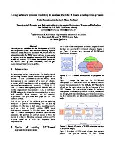
As organizations advance, formal modeling and simulation act as a solid approach for quantitatively understanding their software development processes. This allows CMM level 4 achievement. Drappa and Ludewig (1999) offer some insight in fine-grained simulation and quantitative modeling while Barros et al. (2000a) present a model that supports operational project management. Finally, software project modeling can be used to test process improvement alternatives before implementing them. This allows organizations to reach the ultimate CMM level. Madachy (1994) exemplifies this approach by presenting a model that evaluates the impact of inspections upon a software development project behavior. Tvedt (1996) developed a generic incremental software process model, which can be used to “plug-&-play” process improvement models and analyze their impact over the development process. 3 A Software Project Mod el In mid-1980’s, Abdel-Hamid and Madnick (1991) developed a system dynamics software project model, which formalizes the effects of management policies and actions taken during a software development project. Their work has raised the attention to software dynamic behavior modeling and simulation, being followed by several other software project models (Lin and Levary, 1989) (Lin et al, 1997). The model is divided into four major sections covering human resource management, software production, project planning, and control, as shown in Figure 1. Human Resource Mgmt
Software Production
Software Control
Software Planning
Figure 1 – Abdel-Hamid and Madnick’s model sections
The human resource management section accounts for developers participating on a software development project. It handles personnel hiring, firing, and transferring to other projects. Training enhances developers’ experience level, which influences their productivity and the quality of their work. The software production section allocates available developers to several software development activities, such as training, designing, coding, testing, reworking, and quality assurance. This section handles these activities temporal order, team motivation, developers’ exhaustion, and productivity overhead factors, such as communication and rework. The software control section measures software production activities, describing management actions taken according to such measures. This section control overtime work, schedule pressure, and project funding consumption. Finally, the software planning section provides startup values for the software project parameters, such as project size, initial underestimation factor, initial team size, expected conclusion date, among others. This section also controls the high management willingness to hire new developers, depending on project expected conclusion date. Abdel-Hamid and Madnick’s model (1991) was developed using system dynamics. System dynamics (Forrester, 1961) is a modeling technique and language to describe complex systems, focusing on these systems structural aspects. This technique identifies and models cause-effect relationships and feedback loops.
These relationships are described by using flow diagrams composed by four basic elements: stocks, rates, flows and processes. Stocks represent elements that can be accumulated or consumed over time. Its level, that is, the number of elements in the stock, describes a stock at a given moment. Rates describe stock variations, mathematically formulating their raises and depletions in an equation. Processes and flows complement complex rate equations and calculate intermediate model variables. Simulation is the technique that allows model behavior analysis over time. System dynamics uses continuous time simulation, where a simulator clock, representing time in the real world, is advanced in infinitesimal, predetermined time intervals. Model variables are evaluated at the end of each interval, adjusting their behavior over time. Other types of simulation include discrete-event simulation (Ross, 1990), state-based simulation (Harel, 1990), and rule-based simulation (Drappa and Ludewig, 1999). 4 Simulation Mechanisms Raffo et al. (1999) highlight that dynamic software project modeling can be used to answer two fundamental questions: •
What is the best approach for making decisions about process changes?
•
How can the risk associated with potential process alternatives be assessed?
Simulation can answer these questions. Among several simulation types, we highlight timebased, parameter variation and stochastic simulation. Time-based simulation is an analysis mechanism that presents the value of model variables over simulation time. This mechanism registers selected variable values every time the simulator clock is advanced. These values are generally presented as line graphs, where one axis represents time while the other represents a selected variable. Tools implementing time-based simulation may also allow the user to trace back the simulation, changing some variable values in predetermined time instants, and reevaluating model behavior after the changes. This feature is a kind of scenario analysis, where the user is allowed to “change the state of nature” and analyze model behavior after the adjustments. Parameter variation simulation is an analysis mechanism, which evaluates the impact of changes in a model parameter upon the model results. It usually yields a line graph, where the value of the selected parameter, presented in the horizontal axis, is adjusted linearly from a lower to a higher limit, while the vertical axis presents the values of selected model results calculated with the corresponding parameter value. Parameter variation simulation allows the calibration of specific model parameters, determining their best values for the model to reach a given result. It is generally used when the analyst wants to optimize a model result, targeting its value to a predefined goal by changing only the selected parameter. Stochastic simulation is a mechanism to evaluate non-deterministic models. These models, also called stochastic models, allow the representation of the uncertainties of their variables values. Due to these variable uncertainties, every time a non-deterministic model is evaluated, even if the same model parameters are given, its behavior may change. One way to describe a variable uncertainty is to define its value as a probability distribution function, instead of a crisp numeric value. The uncertainty expressed in a model parameter is propagated throughout the model equations, reaching the model results. Like model parameters, results are also described by a probability distribution function, instead of a crisp number. Monte Carlo simulation (Vose, 1996) is a mechanism that allows the determination of a model results’ probability distribution function based on model parameters distribution. It involves evaluating the same model hundreds or thousands times each time generating a random number for each parameter described as a distribution. Each evaluation calculates a different value for each model result. After several executions, these results can be organized as a frequency histogram, which is a graphical representation of the number of times each value was resulted in a simulation. Normalized, such that the area under the curve reduces to one, the histogram can be understood as the model results’ probability distribution function.
Time-based and parameter variation simulation can be used to evaluate the first question proposed by Raffo et al. (1999). Given separate models for several process improvement alternatives, these models can be evaluated to determine the best solution. An utility function (Hall, 1998) to determine what is the best solution among the alternatives can be defined as a function of model results, such as cost, schedule compression factor, and quality factors. Complementing the previous approaches, stochastic simulation answers the second question, measuring the risk of applying a particular process improvement technique. Process improvement models are subjected to Monte Carlo simulation, evaluating the utility function on each independent run. Since model parameters are described as probability distribution functions, their composed utility function can also be represented as such. The standard deviation of this distribution can be used as a measure of the process improvement alternative risk, explaining how far and how often the alternative resultant behavior can deviate from its expected results. 5 A Simulation Example To illustrate how different simulation approaches can be used for software process quality evaluation and prediction, we will use the Abdel-Hamid and Madnick’s model (1991) and the ILLIUM tool (Barros et al., 2000b) to run and discuss some examples. The ILLIUM tool was developed to allow time-based, parameter variation and stochastic simulation over system dynamics models. For the following examples, consider a development project whose size was initially estimated by its manager as 45.000 lines of code. Consider that the estimation was incorrect, for the project real size is about 64.000 lines of code. Thus, project size was underestimated by a 30% factor. Consider that the organization process allows the manager to determine project effort amount for quality assessment activities. Also, the manager has some freedom to build its initial development team. The following examples illustrate how simulation techniques can help the manager in the decision-making process. The first example studies the application of time-based simulation to predict project schedule according to different initial development team sizes. The second example examines how stochastic simulation can be used to measure project schedule risk due to the initial size underestimation factor. Finally, the last example uses parameter variation simulation to analyze the impact of quality assessment efforts upon project cost. 5.1 Project Schedule Predic tion To determine its initial development team size, the manager uses the COCOMO technique (Boehm, 1981), considering the underestimated project size, that is, 45.000 lines of code. The technique indicates that the project needs 2.360 man-days to be concluded, and that it can be accomplished in 296 days with a 4-person full-time development team. As the organization usually allocates developers for two projects at a time, the desired team would be composed of 8 half-time developers. The manager is interested in analyzing the project behavior making different configurations for the initial development team. There is some freedom for the project’s initial team. Moreover, if more personnel are needed during project development they might be hired from external sources. New developers will have to be trained in the technologies applied to the project and in the organization domain. From previous projects experience, the manager considers that, during training period, new developers’ productivity is half of the experienced developers’ one. Also, their work is more errorprone, conveying more errors per line of code. These values are represented in the model further used for simulations. Suppose that the project starts with four half-time experienced developers and the team enlarges during project life cycle. The manager maintains the initially estimated conclusion date as a project target. Figure 2 plots the expected conclusion date for the project along its life cycle. The conclusion date is measured in days from project start, being presented in the vertical axis. Simulation time, also measured in days, is presented in the horizontal axis.
The graph in Figure 2 is composed of two classes of activities: development and testing. Development activities comprise designing and coding, while testing activities comprise verifying and correcting. The transition between these classes of activities is perceived as the graph slope changes. As presented in the graph, the initial expected conclusion date, 296 days, is maintained as a Figure 2 – Example project expected conclusion date target during about 125 days. As development progresses, new requirements are discovered and developers’ productivity is lower than expected. Perceiving that the project size is greater than initially estimated, management adjusts the project plan to its status, hiring new developers to accomplish the remaining tasks. As a result from the new requirements and team modifications, the expected conclusion date moves to a higher level. Later, delays from testing and reworking activities modify even more the conclusion date, which reaches about 450 days. Observing the graph in Figure 2, the manager decides to analyze the original initial team configuration: an 8-person half-time team. Figure 3 plots the expected conclusion date for the same project, but with an initial 8-person team. Again, the vertical axis presents the expected conclusion date and the horizontal axis presents simulation time, both measured in days. The graph in Figure 3 presents a smoother project accomplishment date evolution along the development process. The initial conclusion date, 296 days, is still maintained for 125 days, when new requirements are discovered, fulfilling the 30% underestimation factor. As management adjusts for these requirements, the conclusion date raises to about 350 days. This “less than linear” conclusion date evolution is better than the 150% Figure 3 – Example project expected conclusion date schedule growth (296 days to 450 days), provided with an 8-persons initial development team by the 4-person initial development team case. Work force distributions along project life cycle for both initial team contexts are showed in Figure 4. The left-hand graph considers an initial 4-person development team, while the right-hand graph considers an 8-person team. In both graphs, the vertical axis represents the number of developers in the project team over simulation time and the horizontal axis displays simulated development time in days.
Figure 4 – Workforce evolution during life cycle for the example project in two scenarios of initial team
As it occurs in the conclusion date graphs, the 8-person development team case has a smoother behavior: the development team is more stable and less inexperienced developers participate in the project. The 4-person initial team case shows a rapid growth in the development team, accomplished by hiring external developers with lower experience in the course of the project. Since the productivity of inexperienced developers is lower than experienced developers and their work is more error-prone, average quality and productivity increase when an 8-person initial team performs the project. Such modifications impact the expected conclusion dates.
Figure 5 shows two graphs demonstrating work distribution along project life cycle for both previous contexts. The horizontal axis presents simulation time, measured in days. Work distribution, presented in the vertical axis as a percentile, is intended to be a portion of a workday that team normally accomplishes at the project. The model assumes that a workday comprises 8 work-hours, where 40% of this time is spent in non-software development activities, such as meetings, telephone calls, coffee breaks, and so on. These activities are generically called slack time. So, developers normal work rate is about 60% of workdays, or 0.6 workdays.
Figure 5 – Work force work distribution for the example project in two scenarios of initial team
The left-hand graph presents the 4-person initial development team case. As management perceives that the conclusion date will overrun project initial schedule, it pressures the development team to work harder. This overwork is first accomplished by reducing slack time, than working more than 8-hours a day. In the example, developers work rate raises up to 1.1 workdays. However, this work rate cannot last forever. As developers exhaust from extra work, they stop overworking, returning to their normal work rate. Only after a normal work rate period the development team will be willing to overwork again. The right-hand graph in Figure 5 has a smoother slope, where the normal work rate is broken when development team attempts to handle undiscovered requirements without extending the project schedule. As team perceives it will not be possible to keep the planned schedule normal work rate is restored and schedule is extended. 5.2 Project Schedule Risk M anagement This section illustrates how project schedule risk can be measured by stochastic simulation. For instance, we will analyze the effects of the uncertainty about the project size underestimation factor upon the project conclusion date. To accomplish this task, we model the underestimation factor as a normal probability distribution function, with 30% mean and 5% standard deviation. This distribution means that in 68% of the simulations the underestimation factor will be between 25% and 35% of the project size. The graphs in Figure 6 show the probability distribution functions for the conclusion date of the example project after 1.000 Monte Carlo simulations.
Figure 6 – Distribution for the conclusion date of the example project with 4-person and 8-person initial teams
The above histograms display several bars, each representing an expected conclusion date range measured in days from project start. Due space limitation reasons, only the upper limit for some bars range is represented in the labels of the horizontal axis. The vertical axis represents the percentile of simulations resulting in a respective conclusion date range. For instance, the first bar of the left-hand graph shows that only about 0.5% of the simulations, that is, 5 simulations, resulted in a conclusion
date lower than 439 days. The next bar shows that only about 2% of the simulations resulted in a conclusion date between 439 and 454 days, and so on. The left-hand graph presents the expected conclusion date distribution for the project in the 4 half-time person initial team case. As we can observe in this graph, project instability, as perceived in the preceding case studies, reflects itself in a highly volatile conclusion date distribution. Within this context, conclusion date ranges (horizontal axis) indicate that the project may last from 439 to 715 days. The average conclusion date is around 576 days, with 89.5 days for standard deviation, which means 68% probability that the project will take between 486 and 665 days to be concluded. The right-hand graph presents the stability and lower risk provided by a more solid and experienced development team. The project conclusion date variation interval is reduced, varying from 346 to 354 days. Its average value is about 349 days, with only 3 days as standard deviation, granting the project 68% probability to be accomplished between 346 and 352 days. 5.3 Impact of Quality Asses sment upon Project Cost This section illustrates how parameter variation simulation can be used to analyze the best workforce allocation for quality assessment activities, measured as a fraction of the total project effort. Project effort is measured in man-days. Suppose we are interested in evaluating workforce allocation impact upon project cost, also measured in man-days. Thus, we want to find the workforce allocation factor which results in lower project cost. Figure 7 shows a graph representing the expected project cost (vertical axis) plotted against workforce allocation factor for quality assessment activities (horizontal axis). The allocation varies from 0% to 40%. The lower limit represents the situation where no quality assessment activities are applied during project development. The upper limit represents a project where 40% of the total effort is dedicated to quality assessment. The graph shows that the optimal allocation is about 18% of the total project effort. If too much effort is dedicated for quality assessment activities, development and testing activities will require more workforce to be accomplished, increasing project cost. If lower effort is dedicated for quality assessment activities, more errors will pass undetected from design to coding, extending testing and correcting activities, and, therefore, increasing project cost. The optimal allocation for quality assessment activities is thus Figure 7 – Project cost plotted against workforce defined as the point with the best trade-off between allocation to quality assessment activities error detection and error discovering and fixing efforts. 6 On Going Works This paper presented three simulation approaches and some applications of them in software process quality evaluation and prediction. A modeling technique, a simulator tool, and a project model where introduced and used as example basis. This work is part of a major research, which comprises scenario based project management, a new paradigm for project management based on formal modeling, simulation, and risk management. Its techniques address the problem of transforming system dynamics project models into operational models, which can be used for project management, status monitoring, and project behavior evaluation throughout the development process. One major difficulty, which inhibits the operational use of dynamic models, is related to the model complexity due its low abstraction level representation. Abdel-Hamid and Madnick’s model (1991) is composed by more than 270 equations. These equations are hard to understand and change. Moreover, the original model includes several simplifications, which inhibits its utilization in operational project management. Fine-grained modeling to resolve such simplifications would raise
model complexity even more. To reduce these difficulties we propose a high level description for project model, which can be translated to system dynamics to be simulated. The project manager will develop his model in a high level representation, execute a program to translate it to system dynamics, and use a simulator to analyze its behavior. The original Abdel-Hamid and Madnick’s model does not allow a project manager to express the uncertainty upon his project parameters. We have implemented Monte Carlo simulation and allowed the manager to describe model parameters as normal probability distribution functions. We intend to expand this capability to include other distributions, such as beta, lognormal, and discrete values. Finally, our major effort intends to create scenario integration API. Scenarios are separate abstract models to represent events, policies, procedures, actions, and strategies that cannot be considered part of a development project, but practices imposed or applied to the project and exceptional situations the manager might encounter during project development. Scenarios are called abstract models, since they must be integrated to a project model, generated from the high level representation, to be simulated. Scenarios represent a reusable knowledge project base to project managers. They allow formal documentation of assumptions and proven information about project elements and their relationship. This information can be reused by projects associated to these elements. During application development, when a project manager determines the current application domain, technologies to be applied during the development, developer roles, artifacts to be built, and so on, these elements associated scenarios help the manager to explore project uncertainties. The ILLIUM tool is available to use and supports part of this whole approach. Managers, developers and researchers interested in trying these ideas in their projects are encouraged to contact the authors by e-mail requesting the tool. Future papers will report results from case studies that are planned to evaluate the feasibility of using such approach in real projects. References Abdel-Hamid, T., Madnick, S.E. (1991) Software Project Dynamics: an Integrated Approach, Prentice-Hall Software Series, Englewood Cliffs, New Jersey Barros, M.O., Werner, C.M.L., Travassos, G.H. (2000a) Applying System Dynamics to Scenario Based Software Project Management, To be presented IN: The Proceedings of the 2000 International System Dynamics Conference, Berghen, NW (August) Barros, M.O., Werner, C.M.L., Travassos, G.H. (2000b) “ILLIUM: Uma Ferramenta de Simulação de Modelos Dinâmicos de Projetos de Software”, Accepted to be published in The Proceedings of the Tools Section of the XIV Brazilian Symposium on Software Engineering, João Pessoa, BR (October) Boehm, B.W. (1981), Software Engineering Economics, Englewood Cliffs, NJ: Prentice-Hall, Inc. Christie, A.M. (1999) “Simulation in Support of CMM-based Process Improvement”, The Journal of Systems and Software, Vol. 46, pp. 107-112 DeMarco, T. (1982) Controlling Software Projects, New York, NY: Yourdon Press, Inc. Drappa, A., Ludewig, J. (1999) “Quantitative Modeling for the Interactive Simulation of Software Projects”, The Journal of Systems and Software, Vol. 46, pp. 113-122 Forrester, J.W. (1961) Industrial Dynamics, Cambridge, MA: The MIT Press Forrester, J.W. (1991) System Dynamics and the Lessons of 35 Years, Technical Report D-4224-4, Sloan School of Management, Massachusetts Institute of Technology Hall, E.M. (1998) Managing Risk: Methods for Software Systems Development, IN: SEI Series in Software Engineering, Reading, MA: Addison Wesley Longman Inc. Harel, D. et al. (1990) “STATEMATE: A Working Environment for the Development of Complex Reactive Systems”, IEEE Transactions on Software Engineering, Vol. 16, No. 3 (April)
Lin, C.Y., Levary, R.R. (1989) Computer-Aided Software Development Process Design, IEEE Transactions on Software Engineering, Vol. 15, No. 9, pp 1025-1037 (September) Lin, C.Y., Abdel-Hamid, T., Sherif, J.S., (1997) Software-Engineering Process Simulation Model (SEPS), Journal of Systems and Software, Vol. 37, pp. 263-277 Madachy, R.J. (1994) A Software Project Dynamics Model for Process Cost, Schedule and Risk Assessment, Ph.D. Dissertation, University of South California, CA Maier, F.H., Strohhecker, J. (1996) Do Management Flight Simulators Really Enhance Decision Effectiveness ?, IN: The Proceedings of the 1996 International System Dynamics Conference, Cambridge, MA, (July) Raffo, D.M., Vandeville, J.V., Martin, R.H. (1999) “Software Process Simulation to Achieve Higher CMM Levels”, The Journal of Systems and Software, Vol. 46, pp. 163-172 Rodrigues, A.G., Williams, T. (1996) “System Dynamics in Software Project Management: Towards the Development of a Formal Integrated Framework”, IN: The Proceedings of the 1996 International System Dynamics Conference, Cambridge, MA, (July) Ross, S.M. (1990) A Course in Simulation, New York, NY: Macmillan Publishing Co. Sterman, J.D. (1992) “System Dynamics Modeling for Project Management”, Technical Report, MIT System Dynamics Group, Cambridge, MA Tvedt, J.D. (1996) An Extensible Model for Evaluating the Impact of Process Improvements on Software Development Cycle Time, Ph.D. Dissertation, Arizona State University, Tempe, AZ Vose, D. (1996) Quantitative Risk Analysis: A Guide to Monte Carlo Simulation Modeling, John Wiley & Sons, Inc, New York