Using Quotient Graphs to Model Neutrality in Evolutionary Search Dominic Wilson
Devinder Kaur
Electrical Engineering and Computer Science University of Toledo Toledo, Ohio 43606, USA 419 508 5472
Electrical Engineering and Computer Science University of Toledo Toledo, Ohio 43606, USA 419 530 8146
[email protected]
[email protected]
structures it is sometimes possible to develop a model of evolution that is simpler than using the actual map. Quotient models are one way of using the symmetry in mapping structures to give simpler models without loss of accuracy. In this paper we use quotient sets to model various evolutionary computing problems.
ABSTRACT We introduce quotient graphs for modeling neutrality in evolutionary search. We demonstrate that for a variety of evolutionary computing problems, search can be characterized by grouping genes with similar fitness and search behavior into quotient sets. These sets can potentially reduce the degrees of freedom needed for modeling evolutionary behavior without any loss of accuracy in such models. Quotients sets, which are also shown to be Markov models, aid in understanding the nature of search. We explain how to calculate Fitness Distance Correlation (FDC) through quotient graphs, and why different problems can have the same FDC but have different dynamics. Quotient models also allow visualization of correlated evolutionary drives.
Quotient models are applicable to both encodings and problems. In order to show the wide applicability of our approach, we apply it to a variety of mapping schemes in the literature including OneMax, deceptive trap, needle in haystack coding, parity coding, majority coding [7] and the redundant coding used in Thomason and Soule [11]. The next section looks at the reasoning behind our approach. Through the use of an example, we introduce our method of using quotient sets and graphs for the modeling of genes and genomes. In Section 3 we apply the method to diverse examples and show how it explains correlated evolutionary drives and fitness distance correlations. Section 4 contains conclusions and future work.
Categories and Subject Descriptors I.2.m.c [Computing Methodologies]: Artificial Intelligence – Miscellaneous - Evolutionary computing and genetic algorithms.
General Terms Theory, Measurement.
2. SEARCH NEUTRALITY In this section we use a simple example to detail how a quotient model is obtained, the benefits of such a model and how to calculate a quotient mutation rate matrix and fitness distance correlation from such models. Though the example to be used is a genotype-to-fitness map for a complete problem, it should be noted that quotient models are also applicable to genotype-tophenotype maps, where the map is an encoding (e.g. parity coding) and can be seen as describing a sub-problem.
Keywords Quotient sets, Degenerate Code, Fitness Distance Correlation, Neutral Evolution.
1. INTRODUCTION In many Evolutionary Computing approaches, a genotype-tophenotype map is used to convert populations of genomes that inhabit a search space into expressions that are either fitness values or can be evaluated on further processing as fitness values. The mapping processes used in a variety of EC applications usually have some implicit structure to them. By this we mean it is usually possible to prescribe the map as an algorithm, or to describe the map by use of a concise description, or a meaningful name. In contrast a randomly generated map usually requires a listing of genotypes and the associated phenotypes they represent. The structure of a map can be examined both from the perspective of how it defines genetic neighborhoods and phenotypic selectivity of genes. Due to symmetries inherent in mapping
Table 1 shows a genotype-to-fitness map for a simple problem based on a 3 bit string. We will use this map to illustrate our approach at using quotient models for evolutionary phenomena. Using the example, we can divide the strings into sets that have the same fitness values. The set of string Ω0 = {000,111} have the same fitness value 0; likewise the set of strings Ω1 = {001,010,100} and Ω 2 = {011,101,110} have fitness values 1 and 2 respectively. We will refer to these sets as fitness neutral sets.
Copyright is held by the author/owner(s). GECCO’08, July 12–16, 2008, Atlanta, Georgia, USA. ACM 978-1-60558-131-6/08/07.
2233
neutral set [1] (shown with gray vertices) has as neighbors two strings in set [2] (black vertices) and one string in set [0] (that with the white vertex); We can therefore infer that for all strings belonging to set [1], mutation of a single bit chosen at random leads to the same phenotypic search distribution (i.e. same probability that the resulting mutant string belongs to sets [0] or [2]). It is not difficult to see that even for the six possible 2-bit mutations and the one possible 3-bit mutation the search distributions are identical for all members of [1]. We therefore denote [1] as a set composed of search neutral members.
Table 1: Example mapping of 3-bit strings to fitness values. 3 bit string Fitness 000 0 001 1 010 1 011 2 100 1 101 2 110 2 111 0
Definition: A search neutral set of strings is a set of fitness neutral strings that has the same phenotypic search distribution on mutation.
Assuming m-bit coding, all mapping schemes map 2 m unique strings unto n fitness cases, with n ≤ 2m . We can represent each string and their fitness values as unitary vectors X and Ψ of sizes 2m and ni respectively, with:
By our definition search neutral sets are (proper or improper) subsets of fitness neutral sets. The value of this characterization is that when we know a string belongs to a particular search neutral set, say [0], then we have all the information necessary to understand its fitness and search behavior. We can replace the string with some other randomly chosen member of the same search neutral set and expect identical search behavior. Set [0] is an example where the fitness neural members are not search neutral. On single bit mutation, for instance, string 000 has strings in [1] as neighbors, whereas string 111 has neighbors in [2]. When all members of a fitness neutral set are not search neutral, we divide the fitness neutral set into search neutral subsets, labeling each of them with both the fitness value and some additional lettering, and list the content of each individual set. We thus get [0a] = {000} and [0b] = {111}.
⎧⎪ . X i = ⎨1, i = x ⎪⎩0 otherwise
For instance strings 000 and 101 have integer values 0 and 5 and are represented as vectors: X = {1 0 0 0 0 0 0 0} , and T
X = {0 0 0 0 0 1 0 0}
T
respectively.
The
vector
representation of Ψ is: ⎧⎪ Ψ i = ⎨1, i = fitness . ⎪⎩0 otherwise The unitary vectors representing fitness 0, 1 and 2 are therefore
Another way of looking at search neutrality is to consider each bit of an m-bit binary string being mutated with some fixed probability μ . The search distribution induced by mutation on
respectively: Ψ = {1 0 0} , {0 1 0} , and {0 0 1} . Note T
T
T
the string can be modeled by applying an 2m × 2m mutation rate matrix M on the string with M i , j = μ d ( x , y ) (1 − μ ) m−d ( x , y ) , where
that these representations form basis (i.e. they are linearly independent and span their respective vector spaces). With these representations, we can construct a ni × 2m linear
d ( x, y ) is the Hamming distance between the present string x , and its potential mutated value y . The mutation rate matrix for our example 3-bit system is:
operator, A , that maps strings to fitness values, with Ψ = AX . The definition of such a matrix is: ⎧⎪ Ai , j = ⎨1, if string j maps to fitness i . ⎪⎩0 otherwise
000 000 ⎡ (1 − μ )3 ⎢ 001 ⎢ μ (1 − μ ) 2 010 ⎢ μ (1 − μ ) 2 ⎢ ⎢ M = ⎢ . ⎢ ⎢ . ⎢ . ⎢ 111 ⎢⎣ μ 3
For our example, ⎡ A0,0 ⎢ A = ⎢ A1,0 ⎢ A2,0 ⎣
A0,1 . . A0,7 ⎤ ⎥ A1,1 . . A1,7 ⎥ , A2,1 . . A2,7 ⎥⎦
⎡1 0 0 0 0 0 0 1 ⎤ ⎢ ⎥ = ⎢0 1 1 0 1 0 0 0⎥ . ⎢⎣ 0 0 0 1 0 1 1 0 ⎥⎦ For every row of A , the set of indexes of columns that have a unit value is a fitness neutral set. We will find this matrix representation of mapping useful in explaining search neutrality, which we now discuss.
001
010
μ (1 − μ ) 2 μ (1 − μ ) 2 (1 − μ )3 μ 2 (1 − μ ) μ 2 (1 − μ ) (1 − μ )3
. . . . . .
. . .
111
⎤ ⎥ ⎥ ⎥ ⎥ ⎥ ⎥ ⎥ ⎥ ⎥ ⎥ 3⎥ (1 − μ ) ⎦
μ3
The genotypic search distribution on mutation of a string is MX , where X is the unitary representation of the string. Its phenotypic search distribution Φ X is given by: Φ X = AMX .
Let Φ = AM , for the example, its transpose is:
Figure 1 represents the strings of our example as vertices on a cube. This representation shows the neighborhood structure between strings. It can be seen that each string in the fitness
2234
π ′ : Ω → {Ω′i }1≤i≤n′ if π ≠ π ′ and every set of Ω′j is a union of sets
⎤ 0⎡ μ 3 + (1 − μ )3 3μ 2 (1 − μ ) 3μ (1 − μ ) 2 ⎢ ⎥ 2 2 3 2 3 1 ⎢ μ (1 − μ ) + μ (1 − μ ) (1 − μ ) + 2μ (1 − μ ) μ + 2μ (1 − μ ) 2 ⎥ 2 2 3 2 3 2 2 ⎢ μ (1 − μ ) + μ (1 − μ ) (1 − μ ) + 2μ (1 − μ ) μ + 2μ (1 − μ ) ⎥ ⎢ ⎥ 2 2 3 2 3 μ − μ + μ − μ μ + μ − μ (1 (1 ) (1 ) 2 (1 ) μ )3 + 2 μ 2 (1 − μ ) ⎥ − ⎢ ΦT = ⎢ 2 2 3 2 3 2 4 μ (1 − μ ) + μ (1 − μ ) (1 − μ ) + 2μ (1 − μ ) μ + 2μ (1 − μ ) ⎥ ⎢ ⎥ 2 2 3 2 5 ⎢ μ (1 − μ ) + μ (1 − μ ) μ + 2 μ (1 − μ ) (1 − μ )3 + 2 μ 2 (1 − μ ) ⎥ ⎢ ⎥ 6 ⎢ μ (1 − μ ) 2 + μ 2 (1 − μ ) μ 3 + 2 μ (1 − μ ) 2 (1 − μ )3 + 2 μ 2 (1 − μ ) ⎥ 3 3 2 2 ⎥⎦ 7 ⎢⎣ μ + (1 − μ ) 3μ (1 − μ ) 3μ (1 − μ )
of Ωi . π ′ is said to be coarser than π . What we are interested in is obtaining the coarsest search neutral sets. The finest partitioning is achieved by having every partition contain a single string only. The coarsest partitioning can be found by grouping together the search neutral subsets of fitness neutral sets. [0b]
We see, from its transpose, that the phenotypic search distribution for columns 1, 2 and 4 of Φ are identical and equal to:
[2]
⎡ μ (1 − μ ) 2 + μ 2 (1 − μ ) ⎤ ⎢ ⎥ 3 2 ⎢ (1 − μ ) + 2μ (1 − μ ) ⎥ . 3 2 ⎢ μ + 2 μ (1 − μ ) ⎥ ⎣ ⎦ This concurs with our visual analysis of search neutrality. Likewise we can observe the identical search distributions for columns 3, 5 and 6 associated with set [2], and the different search distributions of columns 0 and 7 meaning [0a] and [0b] have different search distributions.
[1] [0a] Figure 2: Quotient adjacency graph for 3-bit string example.
A quotient set of search neutral strings is a set having each search neutral set represented by a single member. We can represent quotient set assignment of strings by a matrix Q where:
2.1 Search Neutral Sets As Quotient Sets And Graphs
Let π : Ω → {Ω i } represent the partitioning of strings into
⎧⎪ Qi , j = ⎨1, if integer j maps to search neutral set i . ⎪⎩0 otherwise For our example:
pairwise disjoint and nonempty search neutral sets Ωi , with ∪Ωi = Ω . Because members of each set Ωi have the same search distribution, the partitioning π , is such that for any two partitions Ωi , Ω j , the number of neighbors of any string x ∈ Ωi
7 0⎤ ⎥ 1⎥ 0⎥ ⎥ 0 ⎥⎦ The adjacencies between search neutral sets can be displayed with the aid of quotient sets. To obtain the adjacencies we can take any member of each search neutral set and find their search
to Ω j is independent of the exact value of the string and depends
[0a] [0b] Q= [1] [2]
only on the partition indexes i and j . Such equitable partitioning is a well known concept in graph theory and system aggregation theory [1], [2], [3], [4]. The search neutral members x ∈ Ω i are an equivalence class. Any member can be chosen as a class representative. 110
100
[2]
010
[0]
[1] 000 [0] 001 [1]
2 0 0 1 0
3 0 0 0 1
4 0 0 1 0
5 0 0 0 1
6 0 0 0 1
matrix of the hypercube respectively. If H contains all adjacencies specified by H , then assigning any string X to its search neutral set, QX , and then applying the quotient adjacency matrix should be equivalent to finding its adjacency on the hypercube, HX , and then assigning the result to search neutral sets, i.e.
111
101
1 0 0 1 0
distribution for single bit mutations. Alternatively let H and H represent the quotient adjacency matrix, and the adjacency
[2]
[1]
0 ⎡1 ⎢ ⎢0 ⎢0 ⎢ ⎢⎣0
HQX = QHX ,
011
this yields:
[2]
H = QHQT (QQT ) −1 . The product QQT is a square diagonal matrix with diagonal elements equal to the number of strings within the relevant search neutral set. Thus QQT is full rank and invertible and H always exists. The following matrix represents the adjacencies between search neutral sets for our 3-bit example:
Figure 1: Strings and their fitness [in bracket] represented as vertices on a cube
In general there is more than one way of achieving such partitioning at different levels of fineness (or coarseness). A partitioning π : Ω → {Ωi }1≤i≤n is finer than another partitioning
2235
[0a] H=
[0b] [1] [2]
[0a ] ⎡ ⎢0 ⎢ ⎢0 ⎢ ⎢1 ⎢ ⎣⎢ 0
The off-diagonal elements of M represent nontrivial search. These can be divided into a group that project non-neutral search, and another that project nontrivial neutral search. The diagonal members represent both trivial mutation and lack of mutation. If the search neutral sets are identical with the fitness neutral sets (i.e. Q = A ) then we can refer to M as a phenotypic mutation rate matrix, similar to the phenotypic mutation rate of Poli and Galvan [7]. For our example the quotient mutation rate matrix is:
[0b] [1] [2] ⎤ 0 3 0⎥ ⎥ 0 0 3⎥ . ⎥ 0 0 2⎥ ⎥ 1 2 0 ⎦⎥
The elements of the adjacency matrix representing the number of directed adjacent transitions between and within search neutral sets. For instance any member of search neutral set [1] has 1 neighbor in search neutral set [0a], no neighbor in set [0b], no neighbor in set [1] and 2 neighbors in set [2]. The adjacency matrix can be plotted as a quotient adjacency graph (which is a directed multigraph with each search neutral set represented as a vertex). We will refer to the quotient adjacency graph simply as a quotient graph. The quotient graph represents an entire search neutral set as a single representative entity and shows its relation with other search neutral sets; this way the effects of mutation and the interaction of search neutral sets become easier to understand. Figure 2 is the quotient graph for our example. The shading if the nodes in Figure 2 correspond to the nodes on the cube in Figure 1.
[0a ] ⎡ (1 − μ ) ⎢ ⎢ μ ⎢ 3μ (1 − μ ) ⎢ ⎣ 3μ (1 − μ )
M =
[0b]
[1]
μ
μ (1 − μ )
3
[0 a ] [0b ]
3
[1]
2
[2]
2
3
(1 − μ )
[2] 2
μ (1 − μ )
3
μ (1 − μ )
2
3μ (1 − μ )
(1 − μ ) + 2 μ (1 − μ )
3μ (1 − μ )
μ + 2 μ (1 − μ )
2
3
2
⎤ ⎥ ⎥ μ + 2 μ (1 − μ ) ⎥ ⎥ (1 − μ ) + 2 μ (1 − μ ) ⎦ μ (1 − μ )
2
2
3
2
3
2
2
3
2
2.3 Fitness Distance Correlation Jones [5,6] proposed fitness distance correlation (FDC) as a predictive measure of problem difficulty. Given a set F = { f1 , f 2 , f 3 ,... f n } of fitness values corresponding to all n possible strings, and their associated Hamming distances to their nearest optimum D = {d1 , d 2 , d3 ,...d n } , the fitness distance
Since the arcs of quotient graph indicate single bit adjacencies, the number of incoming (or outgoing) arcs for any node of a quotient model based on an n -bit string is equal to n . Also the ratio of the number of string members of two nodes that have adjacencies is equal to the ratio of the number of arcs between them. For Figure 2, for instance, the ratio of the number of arcs between [0a] and [1] is 1:3, which is the ratio of the number of members of both sets.
correlation measure is given by [7]: 1 n ∑ fdc = n i=1
{( f − f )( d − d )} ’ i
i
σ fσ d
where f , d , σ f and σ d are the means and the standard deviations of the fitness and hamming distances respectively.
Figure 2 shows some of the advantages of the quotient representation. One advantage is that we are able to represent the adjacencies of an 8-node cube by a reduced model (a 4-node quotient model for our example). Without the use of search neutral sets, an m-bit genome requires a 2m × 2m matrix to model its behavior at the genetic level. Another advantage is we can visually assess the phenotypic neighborhood structure. For our example (see Figure 3) we see that there is an evolutionary drive towards the central nodes from the outermost nodes of the quotient graph.
The FDC method has been generally successful in predicting problem difficulty [5,6,8] although there are some known weaknesses in its use [9, 10]. According to [5], a problem can be classified in one of three classes, depending of the value of FDC:
2.2 Quotient Mutation Rate Matrix
•
Misleading (FDC ≥ 0.15), in which fitness tends to increase with the distance from the global optimum,
•
Difficult (−0.15 < FDC < 0.15), for which there is no correlation between fitness and distance, and
•
Easy (FDC ≤ −0.15), in which fitness increases as the global optimum approaches.
Poli and Galvan [7] showed that FDC roughly provides an indication of problem difficulty. They also state that in order to obtain more accurate information one needs to consider how a chosen representation translates genotypic mutation rates into phenotypic mutation rates.
We can define a rate matrix based on the quotient representation that represents the dynamics of mutation at the quotient level. Let M represent the quotient rate matrix. For this matrix to exactly model mutation at the quotient level, assigning any string X to its search neutral set, QX , and then applying the quotient rate matrix should be equivalent to carrying out the normal course of mutation, MX , and then assigning the result to search neutral sets, i.e. MQX = QMX ,which yields:
If the map of strings to fitness is expressed as a quotient set of ni nodes, each node having mi members, the FDC can be expressed as: 1
M = QMQT (QQT ) −1
ni
fdc =
We can show that M always exists by using similar arguments to that used for showing that the quotient adjacency matrix always exists. It can be seen that M has the Markov property that, given the present state of a string, the future state is independent of the past.
2236
∑ ( mi ) i =1
ni
{ (
∑ mi f i − f i =1
σ fσ d
)( d − d )} i
,
Eq. 1
with f =
1
ni
ni
∑ ( mi )
∑ ( mi f i ) ,
d =
i =1
i =1
∑ ( mi )
Figure 3(h) and (i) are based on a redundant coding scheme used by Thomason and Soule [11]. Figure 3(h) shows the quotient graph of the coding scheme and Figure 3(i) shows the quotient graph of a genome composed of 3 such genes.
ni
∑ ( mi d i ) , and i =1
i =1
⎛ ⎜ 1 ni σ f = ⎜ ni ∑ mi f i − f ⎜ ∑ ( mi ) i=1 ⎝ i =1
{
1 ni
(
)} 2
⎛ ⎞ ⎜ 1 ni ⎟ ∑ mi d i − d ⎟ , σ d = ⎜ ni ⎜ ∑ ( mi ) i=1 ⎟ ⎝ i=1 ⎠ 1/2
{
(
)} 2
1/2
⎞ ⎟ ⎟ . ⎟ ⎠
The gene of Figure 3(h) is a one of four possible characters {A, X, Y or Z}. On mutation any gene can change into any other gene with equal probability. Note that A = { X , Y , Z } . For Figure 3(i), if the count of A ’s in a genome is larger than the count of all other characters combined, then the fitness of the genome is equal to the count of A ’s. Otherwise the fitness is the length of the string minus the A count. The goal is to obtain a string of either
3. EXAMPLES OF QUOTIENT GRAPHS Figure 3 shows examples of quotient graphs for some encodings and problems. Although many of the examples in Figure 3 are for 3-bit encodings and problems, Figure 3 (b), (c) and (g) are examples on how they can be generalized to the n bit case for majority and parity encodings. Rather than drawing multiple arcs between nodes, it is sometimes more convenient to indicate the number of arcs by a number beside a single arc; this is done for Figure 3 (b), (c), (g) and (i).
all A ’s or no A . For Figure 3(i), A A A , AA A , AAA and AAA represents the 27 , 27, 9 and 1 genomes with no A , one A , two A and three A ’s respectively. These genomes have fitness of 3, 2, 2 and 3 respectively.
3.1 Some Observations from the Examples
Majority coding works as follows: given n bits (assume n is odd so there cannot be an equal number of zeros and ones in a gene), If the number of ones is greater than the number of zeros then the phenotype level is set to 1, otherwise it is set to 0. For the 3-bit majority coding of Figure 3(a), [0a] = {000}, [0b] = {001,010,100}. [1a] = {011,101,110}, [1b] = {111}.
An important fact that quotient graphs reveal is that there is sometimes a preferred directions of evolutionary drive due to random mutations. The drive is independent of fitness values. The arcs in Figure 3 show that there is a net mutational drive from edge nodes towards central nodes for majority, NIH, deceptive trap and OneMax. This drive is present because the arrangement of phenotypes correlates with distances between genotypes. These correlated mutational drives are sometimes the unsuspecting result of the use of highly structured mapping schemes that cause correlations of the effects of random mutations. Note that the optimal values are at the edge nodes for NIH, deceptive trap and OneMax. It has been observed for these problems that the quasispecies shifts from the optimal edge node (at low mutation rates) to, the centre (at high mutation rates) [12]. This shift is due to the increase in the effect of the net mutational drive. The experiments of Thomason and Soule [11] also show the effect of the net mutational drive. Thomason and Soule used genomes composed of 100 genes, rather than the 3 genes example shown in Figure 3(i). Our explanation applies for either case. We can see
Parity coding works as follows: if the number of ones that are in n genotypic bits is an even number, then the bit at the phenotype level is set to 1, otherwise it is set to 0. For the parity coding of Figure 3(c), [0] is the set of all n-bit strings with even parity, [1] is the set of n-bit strings with odd parity. Needle in haystack (NIH) problem: there is a single genome with optimal fitness of 1. All other genomes have the same suboptimal fitness 0. For the 3-bit Needle in haystack genomes of Figure 3(d), [1] = {111}, [0a] = {000}, [0b] = {011,101,110}, [0c] = {001,010,100}. Deceptive trap problem: The fitness is the number of ones in the genome. However if there is no “1” in the genome the fitness is n + 1 for an n -bit genome. For the 3-bit deceptive trap of Figure 3(e), [3] = {111}, [4] = {000}, [2] = {011,101,110}, [1] = {001,010,100}.
from Figure 3(i), that the mutational drive towards A A A is higher than that towards AAA ; consequently we expect the proportion of solutions of form A A A to be higher than that of the form AAA . We also expect the relative proportions to be
OneMax problem: In the case of Figure 3(f), the fitness is the number of “1” in the genome. For the 3-bit OneMax coding of Figure 3(f), [3] = {111}, [0] = {000}, [2] = {011,101,110}, [1] = {001,010,100}.
dependent on the mutation rate, with the proportion of A A A solutions increasing with increased mutation rate. These are some of the findings of Thomason and Soule [11]; however they interpreted the results as a demonstration that an evolutionary system can avoid a more fit solution in favor of a more robust solution, when under pressure for robustness combined with function sets containing redundant genes.
Figure 3(g) shows the OneMax problem implemented with parity encoding. The fitness in this case is the sum of the fitness of the 3 genes that compose the genome. These genes are n-bit strings that are parity encoded.
3.1.1 Same FDC, Different Dynamics
We do not show the quotient graphs for other problems (NIH and deceptive trap) using parity coding. This is due to page limit constraint. The number of nodes and arc labels for these problems are identical to that of the OneMax case; however the node labels are different. The node labels are identical to the labeling of Figure 3(d) and (e) for NIH and deceptive trap respectively. The quotient graphs for problems using majority coding are more complex and will be detailed in future work.
It can be seen from the OneMax problem based on parity coding that the quotient graph (Figure 3(g)) is similar to that without neutral coding (i.e. Figure 3(f)). This is also true for other problems based on unitation functions. These functions have been found to give the same FDC for different coding sizes as explained in [7]. .
2237
3-bit needle in haystack
3-bit deceptive trap
3-bit OneMax
d
e
f
g
genome of 3 genes based on Thomason and Soule[11]
n-bit parity coding
c
Gene of Thomason and Soule[11]
n-bit majority coding
b
OneMax of 3 genes based on n-bit parity coding
3-bit majority coding
a
h
i
Figure 3: Sample quotient graphs for genes and genomes used in various coding schemes and problems.
The reason why they have the same FDC (though they display different dynamics) is that the ratio between the numbers of members belonging to nodes of the quotient graph is maintained on changing code size. It can be shown (using Eq. 1) that if this ratio is maintained, the FDC is independent of code size. Figure 3(g) shows that the dynamics on using parity coding would be more responsive to changes in mutation rate with larger code size n .
[2] P.F. Stadler, and G. Tinhofer, “Equitable partitions, coherent algebras, and random walks: applications to the correlation structure of landscapes,” MATCH 40 pp.215-261, 2000. [3] C. Godsil, Algebraic Combinatorics, Chapman and Hall, New York, NY. 1993. [4] M. Shpak, P. F. Stadler, G. P. Wagner, and J. Hermisson. “Aggregation of variables and system decomposition: application to fittness landscape analysis,” Theory in Biosciences 123: 33-68, 2004.
4. CONCLUSION AND FUTURE WORK
[5] T. Jones and S. Forrest “Fitness Distance Correlation as a Measure of Problem Difficulty for Genetic Algorithms”, Proceedings of the Sixth International Conference on Genetic Algorithms. pp. 184-192, 1995.
We have used quotient graphs for modeling neutrality in evolutionary search in a variety of evolutionary computing problems. We have shown that search can be characterized by grouping genes or genomes with the same phenotype and search behavior into quotient sets. These sets have been shown to reduce the degrees of freedom needed for modeling evolutionary behavior without any loss of accuracy in such models. We have also shown how to calculate Fitness Distance Correlation (FDC) through quotient graphs, and why different problems can have the same FDC but show different dynamics. Quotient models have been shown to allow visualization of correlated evolutionary drives.
[6] T. Jones.: Evolutionary Algorithms, Fitness Landscapes and Search. PhD thesis, University of New Mexico, Albuquerque (1995). [7] R. Poli and E. Galvan “On the Effects of Bit-Wise Neutrality on Fitness Distance Correlation, Phenotypic Mutation Rates and Problem Hardness”, FOGA 2007. [8] Tomassini, M., Vanneschi, L., Collard, P., Clergue, M.: A study of fitness distance correlation as a difficulty measure in genetic programming. Evolutionary Computation 13(2), 213–239, 2005. [9] B. Naudts and L. Kalle “A comparison of predictive measures of problem difficulty in evolutionary algorithms”. IEEE Transactions Evolutionary Computation 4(1), 1–15, 2000.
In future work we will show how quotient graphs can be used to explain evolutionary phenomena that are difficult to understand without its use. This will include tracking complex population flows on evolutionary landscapes and showing the distributions of complex quasispecies. We will also apply quotient graphs to FDC counterexamples in the literature.
[10]L. Altenberg, “Fitness distance correlation analysis: An instructive counterexample”, Proceedings of the Seventh International Conference on Genetic Algorithms, San Francisco, CA, USA, 1997, pp. 57–64. Morgan Kaufmann Publishers Inc. San Francisco, 1997. [11]R. Thomason and T. Soule “Redundant genes and the evolution of robustness”, Proceedings of the 8th annual conference on Genetic and evolutionary computation. Seattle, Washington, USA pp. 959 – 960, 2006.
5. REFERENCES [1] D. Cvetkovic, P. Rowlinson, and C. Simic, Eigenspaces of Graphs. Encyclopedia of Mathematics and its Applications, Vol. 66, Cambridge University Press, 1997.
[12]N. Richter, J. Paxton and A. Wright. EA Models and Population Fixed-Points Versus Mutation Rates for Functions of Unitation. GECCO 2005, Genetic and Evolutionary Computation Conference. June 2005.
2238