Using Remote Sensing Data to Parameterize Ice ... - Semantic Scholar

water Article

Using Remote Sensing Data to Parameterize Ice Jam Modeling for a Northern Inland Delta Fan Zhang *, Mahtab Mosaffa, Thuan Chu and Karl-Erich Lindenschmidt Global Institute for Water Security, Saskatoon, SK S7N 3H5, Canada; [email protected] (M.M.); [email protected] (T.C.); [email protected] (K.-E.L.) * Correspondence: [email protected]; Tel.: +1-306-881-6508 Academic Editor: Hongjie Xie Received: 27 January 2017; Accepted: 23 April 2017; Published: 27 April 2017

Abstract: The Slave River is a northern river in Canada, with ice being an important component of its flow regime for at least half of the year. During the spring breakup period, ice jams and ice-jam flooding can occur in the Slave River Delta, which is of benefit for the replenishment of moisture and sediment required to maintain the ecological integrity of the delta. To better understand the ice jam processes that lead to flooding, as well as the replenishment of the delta, the one-dimensional hydraulic river ice model RIVICE was implemented to simulate and explore ice jam formation in the Slave River Delta. Incoming ice volume, a crucial input parameter for RIVICE, was determined by the novel approach of using MODIS space-born remote sensing imagery. Space-borne and air-borne remote sensing data were used to parameterize the upstream ice volume available for ice jamming. Gauged data was used to complement modeling calibration and validation. HEC-RAS, another one-dimensional hydrodynamic model, was used to determine ice volumes required for equilibrium jams and the upper limit of ice volume that a jam can sustain, as well as being used as a threshold for the volumes estimated by the dynamic ice jam simulations using RIVICE. Parameter sensitivity analysis shows that morphological and hydraulic properties have great impacts on the ice jam length and water depth in the Slave River Delta. Keywords: river ice; modeling; RIVICE; MODIS; the Slave River Delta

1. Introduction In cold regions, the ice regime of rivers can be divided into three main phases during the winter: river freeze-up, continuous solid ice cover, and ice cover breakup. With ice cover breakup, rubble ice in rivers can pose threats to infrastructure adjacent to the river via jamming and subsequent flooding. However, some ecosystems, particularly inland deltas (e.g., the Slave River Delta), rely on ice jam flooding for replenishment of moisture and sediment. One of the main contributions of flow in the Slave River is from the Peace River. Ice jam development can be separated into three phases: formation, extension, and release. Studying ice jam processes can help extend our understanding of flooding and drying behaviors in river deltas such as the Slave River Delta. Ice jams have rough undersides, which increase flow resistance leading to backwater effects. Within the ice jam, cohesion is a force due to additional freezing which can uphold the structural integrity of the ice jam. Beltaos applied the Rising Limb Analysis Method (RLAM) to analyze hydrodynamic forces in the lower Mackenzie River [1]. He found that pre-breakup conditions, such as Cumulative Melting Degree Days, as well as the rate of flow increases, are important factors in ice jam formation and release. He substantiated these findings with a hydrodynamic model for simulating ice jam waveforms. River ice jamming and subsequent flooding can significantly impact local aquatic ecosystems [2]. On the other hand, the reduced frequency of ice-jam flooding can lead to drying trends and subsequent shifts in flora and fauna composition and succession. Beltaos stated the effects of flow regulation by Water 2017, 9, 306; doi:10.3390/w9050306

www.mdpi.com/journal/water

Water 2017, 9, 306

2 of 18

the dam construction on the river and climate change factors with respect to the drying trends in the Peace-Athabasca Delta [3]. Based on calculations under different flow conditions, he concluded that regulation is the dominant contributor to the lower frequency and severity of ice jam flooding. Prowse and Conly pointed out that ice-jam-induced backwater flowing into the Peace-Athabasca Delta [4] is a major source of that delta’s water supply. Although the Slave River Delta is approximated 400 km downstream of the Peace-Athabasca Delta, and its flows are augmented by the Lake Athabasca and the Athabasca River systems, flow regulation may still affect the Slave River Delta [5]. Inland deltas are particularly susceptible to ice jamming and subsequent flooding. Examples include flooding along the Peace-Athabasca Delta [6], and the lower Red River in Manitoba [7]. To understand the formation and development of ice jams and the flood hazard they induce, the river ice hydraulic model RIVICE was implemented and calibrated to determine the conditions required for ice jamming. RIVICE has proven to be an effective tool for predicting ice jam formation and its impacts on flooding [8]. Due to safety issues, it is difficult to carry out field measurements on ice jams. To obtain the information necessary for better understanding river ice processes, researchers have taken advantage of satellite remote sensing technology, such as MODIS and RADARSAT-2, to monitor and characterize river ice behavior [9]. RADARSAT-2, which is a commercial Earth observation radar satellite, was launched in December 2007 to monitor the environment for natural resource management. It provides high-quality data of the earth’s surface features with a finer resolution (2 m/8 m) but at longer revisit intervals (24 days) than MODIS [10]. Due to the longer wavelength emitted and received by the sensor, an advantage of RADARSAT-2 is that image acquisition is not hindered by weather conditions. Lindenschmidt et al. used RADARSAT-2 to measure ice thickness along the Red River, and determined the relationship between snow depth, ice thickness, and backscattering signal [11]. Due to the high penetration and resolution of RADARSAT-2 signals, it is possible to analyze ice types based on RADARSAT-2 backscatter. Chu and Lindenschmidt classified river ice types using RADARSAT-2 imagery [12]. In another study of the Slave River, different breakup patterns were tracked along the river, using RADARSAT-2 satellite imagery [13]. These researchers used space-borne remote sensing technology (RADARSAT-2 and MODIS) to determine ice extent and ice types. However, it is difficult to acquire ice cover data along the Slave River in consecutive days by RADARSAT-2. Hence, MODIS can be utilized to monitor daily ice changes instead of RADARSAT-2. MODIS (MODerate-resolution Imaging Spectroradiometer) regularly scans the surface of the earth, albeit with a coarse resolution, permitting the monitoring of daily changes in river ice, which is essential for ice cover breakup research [14]. MODIS has been used to facilitate various river-ice-related research, including the determination of the extent of ice and prediction of ice-related hazards along the Susquehanna River [15,16], and ice breakup monitoring on the Mackenzie River [17]. Chaouch et al. designed an automated algorithm to monitor river ice using MODIS data [15]. In addition to river ice data, researchers have also obtained climatic, snow cover and surface temperature data from MODIS products [18–20]. One drawback of MODIS is that it is an optical sensor dependent on cloud cover and daylight conditions. Studies focused on monitoring and modeling ice jams in the Slave River Delta are sparse. Our research goal was to obtain more understanding of river ice formation and deformation processes in the Slave River Delta by focusing on the breakup period during which ice jam flooding is most prevalent. 2. Study Site and Methods 2.1. Study Site The Slave River flows approximately 434 km northward from the Peace River and Peace-Athabasca Delta in Alberta to Great Slave Lake. This study focuses mainly on the delta of the river, the Slave River Delta, which is located at the mouth of the river at Great Slave Lake. The study area of this research

Water 2017, 9, 306

3 of 18

extends from the Jean River to Great Slave Lake, approximately 25 km along the most downstream Water 2017, 9,channel 306 3 of 18 is very part of the main of the river (Figure 1). The drop in elevation at this part of the river low, with a gradient of 0.00003 m/m. The Resdelta Channel is the main channel, from which four other most downstream part of the main channel of the river (Figure 1). The drop in elevation at this part tributaryofchannels, the Middle, Steamboat, and Nagle channels, and the Jean River, branch through the river is very low, with a gradient of 0.00003 m/m. The Resdelta Channel is the main channel, the Slavefrom River Delta. mean annual flow the of the SlaveSteamboat, River is 3400 m3 /schannels, [5]. Regulation of flow by which fourThe other tributary channels, Middle, and Nagle and the Jean the W.A.C Bennett in the reaches ofThe themean Peace Riverflow moderates theRiver seasonal difference in River, branchDam through the upper Slave River Delta. annual of the Slave is 3400 m3/s Regulation of flow by W.A.C Bennett Dam in the upper reaches the Peace River moderates the flow,[5]. typically resulting inthe increasingly low natural winter flowsofand decreasingly high natural seasonal the flow, resulting increasingly natural winter flows and Before summerthe flows. Thedifference ice-coverinseason intypically the Slave River in Delta extendslow from November to May. decreasingly high natural summer flows. The ice-cover season in the Slave River Delta extends from 1980, the frequency of high-magnitude discharge was once every two years; since 1980, this frequency November to May. Before 1980, the frequency of high-magnitude discharge was once every two has beenyears; oncesince every fivethis years [21]. This decreasing trend flood the past several 1980, frequency has been once every five in years [21].frequency This decreasing trend in flooddecades shows the drier conditions in the Slaveshows Riverthe delta. frequency the past several decades drier conditions in the Slave River delta.

Figure 1. The Slave River Delta with important channels. (The dark lines in the bottom panel represent

Figure 1.cross-sections The Slave River channels. (The dark lines500 in and the 1200 bottom spacedDelta 500 mwith apart.important Widths of cross-sections vary between m). panel represent cross-sections spaced 500 m apart. Widths of cross-sections vary between 500 and 1200 m). Geomorphological factors of the river system, such as the sinuosity, channel width, and slope, have a great influence on the river ice regime and, due to its high flows and low gradient, make the Geomorphological factors of the river system, such as the sinuosity, channel width, and slope, Slave River Delta more conducive to ice jam flooding than the rest of the river [22].

have a great influence on the river ice regime and, due to its high flows and low gradient, make the Slave River Delta more conducive to ice jam flooding than the rest of the river [22]. 2.2. Methods 2.2.1. RIVICE Model 2.2. Methods The hydraulic model, RIVICE, was used to simulate ice jamming in the Slave River Delta.

2.2.1. RIVICE RIVICEModel is a one-dimensional model based on the continuity and full dynamic wave equations of flow

momentum. Although there are some limitations in one-dimensional models, they are widely Theand hydraulic model, RIVICE, was used to simulate ice jamming in the Slave River Delta. RIVICE used and have proven to be reasonably accurate. RIVICE can be used to simulate ice processes such is a one-dimensional model based on the continuity and full dynamic wave equations of flow and as frazil ice generation, ice lodgment, ice cover progression through juxtaposition, ice deposition, momentum. Although there are limitations inice one-dimensional hanging dam formation, and some telescoping leading to thickening [23]. models, they are widely used and have proven to be reasonably accurate. RIVICE can be used to simulate ice processes such as frazil ice generation, ice lodgment, ice cover progression through juxtaposition, ice deposition, hanging dam formation, and telescoping leading to ice thickening [23].

Water 2017, 9, 306

4 of 18

The model setup was as follows: Fifty cross-sections of the Slave River spaced 500 m apart (Figure 1) were extracted from a bathymetric model, different parts of which were surveyed between 2013 and 2015 and used to set up the RIVICE model. Cross-sections were also available for the complete reach of the Slave River, approximately 10 km apart, as part of an extensive water surveying campaign carried out in 1980. This campaign included gauging water levels and flows along the main channel and side-channels of the delta. These data served as a basis for calibration and validation of open-water and ice-covered conditions of the flow regime. The gauging stations included the following: Jean River (07NC001), Nagle River (07NC002), and Resdelta Channel (07NC009) (Figure 1). Only water level and flow data from 1980 are available at these stations in the Delta. MODIS data were used to determine ice volumes approximated by: Ice Volume = Average width of ice cover × Ice cover length × Average ice thickness

(1)

All three factors on the right hand of Equation (1) can cause errors in ice volume estimation, which is an input parameter in the RIVICE model. Overestimated ice volume may lead to higher backwater levels. To improve the accuracy of the ice thickness calculation and enhance the reliability of the RIVICE model, aerial photos were used to validate the MODIS ice cover estimation (shown in the Results section). When simulating an ice jam, both the upstream discharge boundary and incoming ice volume data are necessary. For other years, only the discharge data from the Fitzgerald station (07NB001) (Figure 1) can be drawn upon for the ice jam modeling. This station, located in Alberta, has provided continuous daily flow data for the past 68 years [24]. Before running the model, boundary conditions need to be set, particularly the downstream water levels and the upstream discharge. After running RIVICE, simulated water level profiles of the river at different time steps are generated and compared to the gauge data. The fit can be fine-tuned by adjusting the parameter settings. For example, Manning’s coefficient of bed roughness nbed (Table 1) is adjusted until the open water simulations are reasonably in line with recorded water levels. The n8m (Table 1) coefficient can be adjusted to calibrate the roughness along the ice cover underside and match simulated ice-cover conditions with back-water staging observations. Table 1. Parameters used in RIVICE model. Parameters

Description

Units

Hydraulic roughness nbed n8m

River bed roughness Ice roughness

s/m1/3 s/m1/3

Boundary conditions Q W

Upstream discharge Downstream water level

Ice cover characteristics vd ve vice FT PC X

Ice deposit velocity Ice erosion velocity Inflowing ice volume Thickness of ice cover front Porosity of ice cover Ice bridge location (from XS1 in Figure 1)

m/s m/s m3 m — m

Strength properties K1TAN K2

Lateral: longitudinal stresses Longitudinal: vertical stresses

— —

Slush ice characteristics PS ST

Porosity of slush Thickness of slush pans

— m

Note: 1 For water level, m a.s.l. means “meters above sea level”.

m3 /s m a.s.l.

1

Water 2017, 9, 306

5 of 18

Parameters that define the condition and state of the ice regime were also included, such as water temperature, ice cover strength parameters, ice transport parameters and ice cover and flow characteristics. Initial values from the literature and other studies were used to set up the model, but were then adjusted and “fine-tuned” during the calibration process. The model run parameter settings from the Monte-Carlo analysis were chosen for the calibration, as this yielded the best fit between the simulation and observed data. To quantify which factor influences the formation of ice jamming the most, a local parameter sensitivity analysis was carried out to calculate the sensitivity of different parameters on ice jam flooding. Local sensitivity (e) is defined as in [25]: e=

P P O − Oi ∆O (O0 − Oi ) × = × = 0 ∆P O −0.1O0 (P − 1.1P) O0

(2)

in which P refers to the parameter, such as nbed , n8m , etc. (Table 1); O0 is the initial calibrated output variable; and Oi is the output from a change in a parameter value. Sensitive parameters have higher impacts on the output variable and generate higher ∆O values. Some parameters such as inflowing ice volume (vice ), downstream water level, and discharge (Q) are determined by measurements including remote sensing and direct gauge data. Thus, errors from remote sensing data processing may lead to the inaccuracy of the local sensitivity calculation. To improve the accuracy of the analysis, more than one remote sensing technology was utilized in this research. 2.2.2. Remote Sensing Dataset RADARSAT-2 uses microwaves (radar) for ranging and distance measuring. The waves are transmitted obliquely to the normal surface of the earth and the sensor then receives the backscatter signals from features on the surface of the earth which reveal different properties and characteristics of the surface features [26]. After processing these signals, a two-dimensional image can be constructed from which further analyses of the surface or sub-surface features can be made, which, in our case, is the ice cover of the river. Radar data were used to help determining the breakup time of the Slave River, and more importantly, to be compared with MODIS image, improving our understanding of the ice phenology. MODIS is an optical remote sensing satellite sensor. In this study, MOD09GQ (MODIS Surface Reflectance) was applied to assess river ice progression. Since MODIS satellites provide products of daily scans of the earth’s surface, it is possible to acquire a continuous dataset of fine temporal resolution, allowing better tracking of ice cover breakup behavior and potentially identifying factors that cause ice cover retraction [22]. In the MODIS images of the river, brighter pixels represent ice whereas darker ones correspond to open water. The contrast between the light and dark pixels permits the determination of the length of the ice-covered river channel from which ice volume can be calculated. MODIS datasets from 2000 to 2015 were downloaded from the NASA website [27]. Through pixel analyses of the MODIS images, ice cover information can be attained, which are crucial input data for the RIVICE model. ArcGIS [28] was used to pre-process the raw MODIS imagery data and obtain the ice-covered channel length. In ArcMap, the centerline and cross-sections were marked on the MODIS image from which the length of the ice-covered portion was measured. Using these, together with the average ice cover width and estimated ice thickness, ice volume was determined. 2.2.3. Ice Volume Calculation by Using MODIS Various methods for ice volume evaluation have been used, including modeling, direct measurements and the combination of these two [19,29]. We present a novel technique in which remote sensing datasets are applied to calculating the extent of the ice cover and, using an empirical equation to estimate ice thicknesses (h) as a function of both Cumulative Freezing Degree Days (CFDD) and the average channel width in the Slave River Delta, derive an ice volume for downstream ice jamming. After comparing many equations for ice thickness (details about two other equations can

Water 2017, 9, 306

6 of 18

be found in [30]), Stefan’s equation showed the highest consistency with gauged data. Although Water 2017, 9, 306 6 of 18 it is more accurate and reliable to measure the ice thickness using direct measurement or remote sensing sensing technology, technology, the the Stefan Stefan equation equation can can still still reasonably reasonably estimate estimate thermal thermal ice ice growth, growth, even even if if it it does not consider snow depth, which can affect the accuracy of ice thickness calculations. However, does not consider snow depth, which can affect the accuracy of ice thickness calculations. However, while while snow snow depth depth data data were were not not available available for for the the Slave Slave River River Delta, Delta, the the Stefan Stefan equation equation still still provided provided reasonable RADARSAT-2 willwill be utilized for ice estimation in future reasonable ice icethickness thicknessestimates. estimates. RADARSAT-2 be utilized forthickness ice thickness estimation in research to compliment the ice thickness calculation. Plots of the CFDD for all winters from 2000 to future research to compliment the ice thickness calculation. Plots of the CFDD for all winters from 2015 the winter of winter the yearof1980 shown 2. The relationship ice thickness 2000 and to 2015 and the isyear 1980inisFigure shown in Figure 2. Thebetween relationship betweenand ice √ the CFDD is h = c CFDD, where c is a constant. Thawing effects on ice volume can be accounted for thickness and CFDD is h = c√CFDD, where c is a constant. Thawing effects on ice volume can by be ◦ C. Thus, thawing effects determining theby cumulative average air temperature degrees surpassing −5degrees accounted for determining the cumulative average air temperature surpassing −5 °C. were to attenuate CFDD in spring. Thus,used thawing effects were used to attenuate CFDD in spring.

Figure 2. Plots of cumulative freezing degree days for winters (1 October–19 April) between the years Figure 2. Plots of cumulative freezing degree days for winters (1 October–19 April) between the years 1980 and and 2015 2015 at at Fort Fort Smith, Smith, Northwest Northwest Territories. Territories. 1980

MOD09GQ band2 (wavelength: 841–876 nm, resolution: 250 m) datasets were used to establish MOD09GQ band2 (wavelength: 841–876 nm, resolution: 250 m) datasets were used to establish time series to estimate the ice cover situation of the Slave River [31]. Different pixel values in the time series to estimate the ice cover situation of the Slave River [31]. Different pixel values in the MODIS MODIS images represent different backscatters to which threshold values are applied to distinguish images represent different backscatters to which threshold values are applied to distinguish water water from ice. By creating the histogram, the distribution of pixel values for each image can be from ice. By creating the histogram, distribution of signal pixel values each image be determined. determined. Clear water provides the little backscatter to thefor satellite sincecan it absorbs longer Clear water provides backscatter signal to the satellite it absorbs wavelengths and wavelengths and thelittle reflected shorter wavelengths tendsince to scatter in longer the air. Hence, longer the reflected shorter wavelengths tend to scatter in the air. Hence, longer wavelengths appear more wavelengths appear more sensitive to the difference between water and ice. Since MOD09GQ band2 sensitive to wavelength the difference between and ice. Since band2 is longer in wavelength is longer in than band1, water it has been chosen forMOD09GQ our ice phenology research. A heat balance than band1,based it has on been chosen river for our ice phenology A heat how balance calculation basedand on calculation upstream temperature mayresearch. help determine much ice is melting upstream river temperature may help determine how much ice is melting and moving respectively. moving respectively. This calculation requires more extensive field sampling and can be addressed This calculation requires more extensive field sampling can be addressed in future work. Due to in future work. Due to this characteristic of clear water,and it appears dark on MODIS imagery. On the this characteristic of clear water, it appears dark on MODIS imagery. On the other hand, ice provides other hand, ice provides more reflectance and appears lighter than clear water on the MODIS more reflectance appearsleads lighter clear water different on the MODIS imagery [32].MODIS This difference imagery [32]. Thisand difference to than the significantly pixel values in the imagery. leads to the significantly different pixel values in the MODIS imagery. Pixel values, with only one Pixel values, with only one feature variable (a pixel is either ice or water), are normally distributed. feature variable (a pixel is either ice or water), are normally distributed. Theoretically, a mixture of Theoretically, a mixture of two normal distributions forms a bimodal distribution. Figure 3 shows an two normal distributions forms a bimodal distribution. Figure 3 shows an example of the MODIS example of the MODIS pixel-value distribution from 17 November 2002. On that day, both ice and pixel-value distribution from 17 November 2002. On(local that day, both representing ice and waterice appear in thecan river, water appear in the river, so that two distinct peaks maxima) and water be so that two distinct peaks (local maxima) representing ice and water can be found in the histogram, found in the histogram, which is consistent with the bimodal distribution theory. There is a big difference between the pixel values of the ice and water, and a value separating the two establishes the threshold. On cloudy days, backscatter values are difficult or even impossible to attain. Hence ice volumes for those days have to be interpolated between clear-day images [12]. The algorithm Harmonic Analysis of Time Series (HANTS) was used to replace cloud-contaminated pixels with

Water 2017, 9, 306

7 of 18

which is consistent with the bimodal distribution theory. There is a big difference between the pixel values of the ice and water, and a value separating the two establishes the threshold. On cloudy days, backscatter values are difficult or even impossible to attain. Hence ice volumes for those days have7to Water 2017, 9, 306 of be 18 interpolated between clear-day images [12]. The algorithm Harmonic Analysis of Time Series (HANTS) Fourier valuescloud-contaminated from MODIS images [33]. After interpolation, pixel values change so that was usedseries to replace pixels with Fourier series values from MODIS images [33]. another threshold must applied to thesointerpolated Applying threshold tointerpolated the MODIS After interpolation, pixelbevalues change that anotherimages. threshold must bethe applied to the image pixel-value of water ice can be measured aspercentages well as ice volumes. images. Applying distributions, the threshold percentages to the MODIS imageand pixel-value distributions, of water During the ice breakup period, the diminishing ice of the upstream reach is considered and ice can be measured as well as ice volumes. During the ice breakup period, the diminishing to icebe of inflowing ice reach at theisdownstream icebejam. We doice make allowance for the of make the iceallowance front by the upstream considered to inflowing at the downstream icerecession jam. We do tracking the location thefront ice front at a daily resolution using the imagery. Ice motion for the recession of theofice by tracking thetime location of the ice front at MODIS a daily time resolution using velocities the year were approximately 48–100were km/day. Based on48–100 the ice front the MODISinimagery. Ice2000–2015 motion velocities in the year 2000–2015 approximately km/day. movement, ice can be tracked. Oneice point is point that not of the ice is downstream Based on theinflowing ice front movement, inflowing can of beuncertainty tracked. One of all uncertainty that not all of the ice downstream front may be of moving; some be rather, meltingsome while stationary, due while to warm inflow the ice rather, front may be could moving; could be melting stationary, river it water. is veryHowever, difficult itorisperhaps impossible to distinguish much ice how has due towater. warm However, inflow river very difficult or perhaps impossiblehow to distinguish moved from to the delta, as melting the next image A much ice hasupstream moved from upstream toopposed the delta,toasjust opposed to before just melting before thewas nextacquired. image was shorter time interval between image acquisitions would be necessary. acquired. A shorter time interval between image acquisitions would be necessary.

Figure Figure 3. 3. The The histogram histogram of of pixel pixel values values of of MODIS MODIS imagery. imagery.

Ice volume calculation processes are shown in Figure 4 Using the Geographic Information Ice volume calculation processes are shown in Figure 4 Using the Geographic Information System System (GIS) [28], the water surface area of the Slave River Delta was measured, which is 12.8 km2. (GIS) [28], the water surface area of the Slave River Delta was measured, which is 12.8 km2 . Percentages Percentages of the ice cover on the Slave River Delta are calculated from MODIS datasets. An example of the ice cover on the Slave River Delta are calculated from MODIS datasets. An example of calculating of calculating ice percentages is shown in Figure 4. ice percentages is shown in Figure 4. 2.2.4. Data Preparation for Model 2.2.4. Data Preparation for Model Essential inputs to the RIVICE control files include upstream discharge boundaries, downstream Essential inputs to the RIVICE control files include upstream discharge boundaries, downstream water level boundaries, incoming ice volume, the location of ice lodgments, and cross-sectional data. water level boundaries, incoming ice volume, the location of ice lodgments, and cross-sectional data. The water level data can be obtained from gauge stations (Figure 5). Flow data of Resdelta Channel The water level data can be obtained from gauge stations (Figure 5). Flow data of Resdelta Channel (07NC009) (Figure 1) and Fitzgerald station are shown in Figure 6 and were used as the upstream (07NC009) (Figure 1) and Fitzgerald station are shown in Figure 6 and were used as the upstream discharge boundary. The downstream water levels were acquired at Great Slave Lake, which is used discharge boundary. The downstream water levels were acquired at Great Slave Lake, which is used as the boundary condition for modelling according to the daily water level data at Yellowknife Bay as the boundary condition for modelling according to the daily water level data at Yellowknife Bay station (07SB001). station (07SB001).

Water 2017, 9, 306 Water 2017, 9, 306

8 of 18 8 of 18

Figure 4. Steps taken in determining ice cover percentages.

Water 2017, 9, 306 Water Water 2017, 2017, 9, 9, 306 306

9 of 18 99 of of 18 18

Figure open water case of the three gauge stations. Figure 5. 5. Water Water level level data data for for open open water water case case of of the the three threegauge gaugestations. stations. Figure 5. Water level data for

Figure 6. 6. Measured flow flow data at at Resdelta Channel and Fitzgerald Station. Figure Figure 6. Measured Measured flow data data at Resdelta Resdelta Channel Channel and and Fitzgerald Fitzgerald Station. Station.

3. 3. Results Results 3.1. Ice Volume Volume 3.1. 3.1. Ice Ice Volume The CFDD was determined for for each winter from mean daily air temperature records between The The CFDD CFDD was was determined determined for each each winter winter from from mean mean daily daily air air temperature temperature records records between between 1971 and 2015. In the the Stefan equation, equation, the constant constant c depends on on many factors factors such as as meteorological 1971 1971 and and 2015. 2015. In In the Stefan Stefan equation, the the constant cc depends depends on many many factors such such as meteorological meteorological conditions, geomorphological parameters, and water quality. is derived empirically asasthe slope ofof a conditions, √ ItIt conditions, geomorphological geomorphological parameters, parameters, and and water water quality. quality. It is is derived derived empirically empirically as the the slope slope of linear relationship between measured ice thicknesses and CFDD (Figure 7). Based on the field survey aa linear linear relationship relationship between between measured measured ice ice thicknesses thicknesses and and √CFDD (Figure 7). 7). Based Based on on the the field field √CFDD (Figure survey survey and and relationship relationship between between ice ice thicknesses thicknesses and and CFDD CFDD at at the the Slave Slave River River Delta Delta and and its its tributaries tributaries

Water 2017, 9, 306

10 of 18

Water 2017, 9, 306

10 of 18

and relationship between ice thicknesses and CFDD at the Slave River Delta and its tributaries [13], the constant c√ wasc was estimated to beto0.021. The The blueblue trendline shows the the relationship between the the ice [13], the constant estimated be 0.021. trendline shows relationship between thickness andandCFDD of the Slave River near FortFort Smith. TheThe constant c equals 0.018. Hence, 0.020.02 has ice thickness of the Slave River near Smith. constant c equals 0.018. Hence, √CFDD been chosen as the constant, and the trendline with a slope of 0.02 m/m is shown by the orange line in has been chosen as the constant, and the trendline with a slope of 0.02 m/m is shown by the orange Figure 7. line in Figure 7.

Figure Figure 7. 7. Relationship Relationship between between the the cumulative cumulative freezing freezing degree degree days days and and ice ice thicknesses. thicknesses.

After determining ice percentage, ice thickness, and the ice-covered water surface area, ice After determining ice percentage, ice thickness, and the ice-covered water surface area, ice volumes were calculated. volumes were calculated. It is difficult to determine the ice cover extent from MODIS images during cloud-covered It is difficult to determine the ice cover extent from MODIS images during cloud-covered periods, periods, particularly for the breakup events of 2007 and 2010. The ice cover thresholds for these two particularly for the breakup events of 2007 and 2010. The ice cover thresholds for these two years years cannot be determined. Thus, ice volumes cannot be calculated for these two events. Aerial cannot be determined. Thus, ice volumes cannot be calculated for these two events. Aerial photos photos acquired along the Slave River on 29 April 2015 were used to validate the ice volume acquired along the Slave River on 29 April 2015 were used to validate the ice volume estimation result estimation result of MODIS (Figure 8). The RADARSAT-2 image acquired on 30 April was compared of MODIS (Figure 8). The RADARSAT-2 image acquired on 30 April was compared with MODIS data with MODIS data for the same day (Figure 9). The noticeable difference between images from these for the same day (Figure 9). The noticeable difference between images from these two satellites is two satellites is partly due to the different acquisition times, other reasons can be found in [12]. partly due to the different acquisition times, other reasons can be found in [12]. In Figure 10, three ice volume clouds (scatters showing the relationship between ice volumes and In Figure 10, three ice volume clouds (scatters showing the relationship between ice volumes and water levels) are shown. The cluster of blue dots show the modeling results of HEC-RAS, and the red water levels) are shown. The cluster of blue dots show the modeling results of HEC-RAS, and the ones and green ones show RIVICE modeling results with and without thawing effects. Thawing red ones and green ones show RIVICE modeling results with and without thawing effects. Thawing comes into effect for days on which average temperatures are above −5 °C. Clearly, the ice volumes comes into effect for days on which average temperatures are above −5 ◦ C. Clearly, the ice volumes are lower when thawing is incorporated in the calculation. The RIVICE clusters yield lower are lower when thawing is incorporated in the calculation. The RIVICE clusters yield lower backwater backwater elevations than HEC-RAS, which is to be expected, because not every jam that is formed elevations than HEC-RAS, which is to be expected, because not every jam that is formed is expected is expected to be a fully-evolved equilibrium jam as premised by HEC-RAS. In HEC-RAS, stresses to be a fully-evolved equilibrium jam as premised by HEC-RAS. In HEC-RAS, stresses acting on an acting on an ice jam are calculated based on the ice jam force balance equation, while the deposition ice jam are calculated based on the ice jam force balance equation, while the deposition and erosion and erosion of ice covers are not taken into account [23,34]. In RIVICE, ice jam formation and of ice covers are not taken into account [23,34]. In RIVICE, ice jam formation and development were development were considered in a dynamic balance process. considered in a dynamic balance process. The incoming ice volume of 1.1 million m33 will lead to backwater staging effects causing ice jam The incoming ice volume of 1.1 million m will lead to backwater staging effects causing ice jam flooding, which replenishes moisture in the delta during ice-cover breakup. When the incoming ice flooding, which replenishes moisture in the delta during ice-cover breakup. When the incoming ice volume is higher than 1.5 million m33, the backwater effects are substantial. volume is higher than 1.5 million m , the backwater effects are substantial.

Water 2017, 9, 306 Water 2017, 9, 306 Water 2017, 9, 306

11 of 18 11 of 18 11 of 18

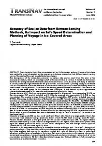
Figure 8. Examples of aerial photographs used to validate the MODIS ice cover estimation (the

Figure 8. Examples of aerial photographs usedused to validate the MODIS ice cover estimation (the(the number Figure 8. Examples of aerial photographs to validate the MODIS ice cover estimation number shows the location of the aerial photos. Data were acquired on 29 April 2015). shows the location of the aerial photos. Data were acquired on 29 April 2015). number shows the location of the aerial photos. Data were acquired on 29 April 2015).

Figure 9. Comparison of RADARSAT-2 (right panel) and MODIS (left panel) image (data were

Figure 9. Comparison of RADARSAT-2 (right panel) MODIS panel) image Figure 9. Comparison of 2015). RADARSAT-2 (right panel) and and MODIS (left(left panel) image (data(data werewere acquired acquired on 30 April on 30 April 2015). on 30acquired April 2015).

Water 2017, 9, 306 Water 2017, 9, 306 Water 2017, 9, 306

12 of 18 12 of 18 12 of 18

Figure 10. Ice volume calculation results from HEC-RAS and RIVICE. Figure from HEC-RAS HEC-RAS and and RIVICE. RIVICE. Figure 10. 10. Ice Ice volume volume calculation calculation results results from

3.2. Model Calibration 3.2. Model Calibration 3.2. Model Calibration Water levels from 1980 recorded during the open-water and ice-covered period were used to Water levels from 1980 recorded during the open-water and ice-covered period were used to Water from 1980 recorded during the open-water and ice-covered period were used to calibrate thelevels RIVICE model. calibrate the RIVICE model. calibrate RIVICE model. In 1980, during the open-water period, the daily flow reached a Openthewater conditions: Open water conditions: In 1980, during the open-water period, the daily flow reached a Open water conditions: 1980, during the 6), open-water the daily flow reached maximum 3 maximum of 4870 m 3/s, on 13In June 1980 (Figure when theperiod, water level elevation of GreataSlave Lake maximum3of 4870 m /s, on 13 June 1980 (Figure 6), when the water level elevation of Great Slave Lake of 4870 m /s, on 13 June 1980 (Figure 6), when the water level elevation of Great Slave Lake was was 156.43 m [24]. These values were used as the boundary conditions in RIVICE. The minimum was 156.43 m [24]. These values were used as the boundary conditions in RIVICE. The minimum 156.43flow m [24]. Thesethe values used as theinboundary RIVICE. The minimum daily1980. flow daily during openwere water period 1980 wasconditions 2660 m3/s,inwhich occurred on 21 May daily flow during the open water period in 19803 was 2660 m3/s, which occurred on 21 May 1980. during the open water period in 1980 was 2660 m /s, which occurred on 21 May 1980. Comparisons Comparisons of gauged and simulated data are provided in Figure 11, showing good agreement Comparisons of gauged and simulated data are provided in Figure 11, showing good agreement of gauged and simulated data are provided in Figure 11, showing good agreement between the two. between the two. between the two.

(a) (a)

(b) (b)

Figure 11. Calibration for RIVICE simulation under open water conditions: (a) water level profile Figure 11. 11. Calibration for RIVICE simulation under open water conditions: (a) water level profile under minimum daily flow; (b) water level profile under maximum daily flow. under minimum daily flow; (b) water water level level profile profile under under maximum maximum daily daily flow. flow.

The change of water levels at the Jean River gauge (07NC001) occurred approximately one day The change change of water water levels levels at at the the Jean Jean River River gauge gauge (07NC001) (07NC001) occurred occurred approximately approximately one day The one day earlier than at theofNagle Channel gauge (07NC002) and two days earlier than at the Resdelta River earlier than than at at the the Nagle Nagle Channel gauge gauge (07NC002) (07NC002) and and two two days days earlier earlier than than at at the the Resdelta Resdelta River River earlier gauge (07NC009) (Figure Channel 1). gauge (07NC009) (Figure 1). gauge (07NC009)conditions: (Figure 1). RIVICE was also implemented to simulate ice-covered conditions of the Ice-covered Ice-covered conditions: conditions: RIVICE was implemented to simulate ice-covered conditions of of the the Ice-covered RIVICE was also also simulate ice-covered conditions main channel in the Slave River Delta. The implemented water level ofto the Resdelta River gauge (07NC009) main channel channelininthethe Slave River Delta. The water level of the Resdelta River gauge (07NC009) main Slave River Delta. The levelthe of the Resdelta River gauge (07NC009) (Figure 1) (Figure 1) on 31 January 1980, was used towater calibrate model. (Figure 1) on 31 January 1980, was used to calibrate the model. on 31Figure January 1980, was used to calibrate the model. 12 shows good agreement between the modeling result and the gauge recording of Figure 12 12 shows shows good good agreement agreement between between the the modeling modeling result result and and the the gauge gauge recording recording of of Figure Resdelta (07NC009). Resdelta (07NC009). (07NC009). Resdelta

Water 2017, 9, 306 Water 2017, 9, 306 Water 2017, 9, 306

13 of 18 13 of 18 13 of 18

Figure 12. 12. Calibrated Calibrated ice-covered ice-covered water water profile profilefor forthe theSlave SlaveRiver RiverDelta. Delta. Figure Figure 12. Calibrated ice-covered water profile for the Slave River Delta.

Ice-jammedconditions: conditions: Simulatingiceice jams more is more complicated than simulating open water Ice-jammed complicated than simulating openopen water and conditions:Simulating Simulating icejams jamsis is more complicated than simulating water and ice-covered conditions since more factors need to be used in RIVICE calculations to simulate ice ice-covered conditions sincesince moremore factors needneed to betoused in RIVICE calculations to simulate ice jam and ice-covered conditions factors be used in RIVICE calculations to simulate ice jam formation and progression. Water level data at the Great Slave Lake (156.557 m) and the Resdelta formation andand progression. Water level data at at thethe Great Slave jam formation progression. Water level data Great SlaveLake Lake(156.557 (156.557m) m)and and the the Resdelta Channel (156.884 m) on 2727April 1980 were used to set up and calibrate the model, respectively. After Channel (156.884 m) on April 1980 were used to set up and calibrate the model, respectively. (156.884 m) on 27 April 1980 were used to set up and calibrate the model, respectively. After defining the incoming ice volume on ice jam, the water level profile can be determined (Figure 13). After defining the incoming ice volume on the ice water jam, the level can be determined defining the incoming ice volume on ice jam, levelwater profile can profile be determined (Figure 13). Gauged water levels and HEC-RAS modeling results are applied to calibrate the ice-jam modeling (Figure Gauged levels andmodeling HEC-RASresults modeling results are calibrate ice-jam Gauged13). water levelswater and HEC-RAS are applied to applied calibratetothe ice-jamthe modeling results. HEC-RAS is a one-dimensional hydrodynamic model which is mainly used for simulating modeling results. HEC-RAS is a one-dimensional hydrodynamic model which is mainly used for results. HEC-RAS is a one-dimensional hydrodynamic model which is mainly used for simulating steady and unsteady flow routing based on an implicit four-point finite difference scheme. simulating and unsteady flow routing an implicit four-point finitedifference difference scheme. scheme. steady andsteady unsteady flow routing based based on anonimplicit four-point finite The HEC-RAS HEC-RAS model model simulates simulates only only equilibrium equilibrium ice ice jams, jams, i.e., i.e., in in steady steady state, state, not not dynamically, dynamically, as as is is The not the case in RIVICE. Hence, the HEC-RAS result can be seen as the maximum backwater level that can the case in RIVICE. Hence, the HEC-RAS result can be seen as the maximum backwater level that can be determined if the ice jam formation is not limited by the supplyof of incomingrubble rubble ice. be determined if the ice jam formation is not limited by the supply supply of incoming incoming rubble ice. ice.

Figure 13. Simulated ice-jammed water profile for the Slave River Delta. Figure 13. Simulated ice-jammed water profile for the Slave River Delta. Figure 13. Simulated ice-jammed water profile for the Slave River Delta.

Some of the gauges in the delta were installed during the winter, prior to ice-cover breakup. Ice Some of the gauges in the delta were installed during the winter, prior to ice-cover breakup. Ice jamsSome regularly occur along this reach during the final breakup of the Slave River. The error between of the gauges thereach deltaduring were installed prior to ice-cover jams regularly occur alonginthis the final during breakupthe of winter, the Slave River. The error breakup. between simulated values occur and observed ones is shown in Figure 14, which is acceptable. Ice jams regularly along this reach duringin theFigure final breakup of is the Slave River. The error between simulated values and observed ones is shown 14, which acceptable. simulated values and observed ones is shown in Figure 14, which is acceptable.

Water 2017, 9, 306

14 of 18

Water 2017, 9, 306 Water 2017, 9, 306

14 of 18 14 of 18

Figure14. 14.Error Errorbetween between simulated simulated values Figure valuesand andobserved observeddata. data. Figure 14. Error between simulated values and observed data.

Jam Flooding 3.3.3.3. IceIce Jam Flooding 3.3. Ice Jam Flooding Figure showsthe thefloodwater floodwaterextensions, extensions, calculated calculated with the floodplain forfor Figure 1515 shows withHEC-RAS, HEC-RAS,within within the floodplain Figure 15cover showswater the floodwater withand HEC-RAS, the floodplain for the ponding surface atextensions, elevationscalculated of 156, 157, 158 m. within For instance, when the the ponding cover water surface at elevations of 156, 157, and 158 m. For instance, when the backwater the ponding cover water surface at elevations of 156, 157, and 158 m. For instance, when the backwater level exceeds 156 m, the area to the left-hand side of the red line will be flooded. To level exceeds 156 m, the area to the left-hand side of the red line will be flooded. To determine the backwater the level exceeds 156 m, of the to the which left-hand sideflooding, of the red will model be flooded. To determine backwater effects icearea jamming, causes theline RIVICE was run backwater effects of ice jamming, which causes flooding, the RIVICE model was run three times determine backwater effects ofconditions: ice jamming, which causes flooding,and the ice-jammed RIVICE model was run three timesthe under the following open water, ice-covered, conditions. under following the conditions: open water, ice-covered, and ice-jammed conditions.conditions. These three threethe times following conditions: open water, ice-covered, and ice-jammed These three under scenarios were simulated using the same boundary downstream water level elevation scenarios were simulated using the same boundary downstream water level elevation (156.45 m), These three scenarios wereupstream simulated usingflows. the same boundary downstream watersimulated level elevation (156.45 m), but different water Associated with the HEC-RAS flood butextension different upstream water flows. Associated with the HEC-RAS simulated flood extension under (156.45 m),under but different upstream water flows. Associated with the HEC-RAS simulated different backwater levels, the RIVICE modeling results can help determineflood the different backwater levels, the RIVICE modeling results can help determine the maximum possible extension under different levels, the RIVICE results can help determine the maximum possible floodingbackwater extent in the floodplain undermodeling different situations. flooding extent in theflooding floodplain under different situations. maximum possible extent in the floodplain under different situations.

Figure 15. Floodplain under different simulated water levels (HEC-RAS result); Floodplain under Figure Floodplain under different simulated water levels under different simulated water levels (HEC-RAS result).water Figure 15.15. Floodplain under different simulated levels (HEC-RAS (HEC-RASresult); result);Floodplain Floodplain under different simulated water levels (HEC-RAS result). different simulated water levels (HEC-RAS result).

Water 2017, 2017, 9, 9, 306 306 Water

15 of 18

3.4. Local Sensitivity Analysis 3.4. Local Sensitivity Analysis Applying equation (2) to the local sensitivity analysis, e-values are positively proportional to Applying equation (2) to theparameter local sensitivity analysis, e-values are based positively proportional to parameter sensitivity. Given that, sensitivity can be evaluated on e-values. parameter sensitivity. Given that, parameter sensitivity can be evaluated based on e-values. Hydraulic properties, including upstream discharge (Q), downstream water level (W), and the Hydraulic properties, including upstream discharge (Q), on downstream water levelThe (W), and the riverbed roughness coefficient (n ), have the greatest impact the backwater levels. upstream riverbed roughness coefficient (n ), have the greatest impact on the backwater levels. The upstream bed discharge (Q) has the greatest negative impact on the ice jam length. discharge (Q) has the greatest negative on 1) thehave ice jam length. Ice transporting properties (v , impact v , Table little impact on the ice jamming since the Ice transporting properties (v , v , Table 1) have little impact on the ice thecover. main e dep main process of ice jam formation is ice thickening as forces shove andjamming retract since the ice process of ice jam formation is ice thickening as forces shove and retract the ice cover. Surprisingly, ice Surprisingly, ice volume (V ) has some impact on the ice jamming length but not on backwater volume (V ) has some impact on the ice jamming length but not on backwater staging (Figure 16). ice staging (Figure 16).

Figure 16. Local parameter sensitivity analysis result. Figure 16. Local parameter sensitivity analysis result.

Physical properties of the ice (FT, PC, PS, ST) have some influence on the ice jam morphology. Physical properties of the ice (FT, PC, PS, ST) have on theleading ice jamtomorphology. Increasing porosity will increase compaction between ice some blocksinfluence when shoved, a reduction Increasing porosity will increase compaction between ice blocks when shoved, leading to a reduction in ice jam length. An increase in ice front thickness means more surface area is available for water in ice jamon length. increase in icethe front means more surface area is available for of water shoving the iceAn front to retract icethickness jam cover, which corresponds to the shortening the shoving on the ice front to retract the ice jam cover, which corresponds to the shortening of the ice jam. ice jam. The of the the lodgment lodgment X The location location of X has hasthe thelargest largest positive positive impact impact on on the the ice ice jam jam length, length, potentially potentially due to varying cross-section flow dimensions along the river. Moving the location further downstream due to varying cross-section flow dimensions along the river. Moving the location further leads to a decrease and shortening of shortening the ice jam of cover. downstream leads in to backwater a decrease staging in backwater staging and the ice jam cover. Mechanical properties, K1 and K2, have a significant impact on the Mechanical properties, K1 and K2, have a significant impact on the ice ice jam jam length length and and partly partly on on the water level, which is consistent with the research in [35]. Ice cover internal resistance will increase the water level, which is consistent with the research in [35]. Ice cover internal resistance will increase with K1, which with an an increase increase in in K1, which provides provides more more resistance resistance to to shoving. shoving. Therefore, Therefore, more more ice ice can can stay stay in in place and the ice jam length is extended. Greater internal resistance corresponds to less thickening place and the ice jam length is extended. Greater internal resistance corresponds to less thickening of of the the ice ice cover, cover, allowing allowing more more flow flowunderneath underneaththe theice icecover coverand anddecreasing decreasingbackwater backwatereffects. effects. 4. Discussion 4. Discussion Both numerical modeling and remote sensing images are useful tools for studying river ice Both numerical modeling and remote sensing images are useful tools for studying river ice processes. These two methods were combined successfully to characterize ice jamming within the processes. These two methods were combined successfully to characterize ice jamming within the Slave River Delta. The excellent agreement between modeling results and measurement readings Slave River Delta. The excellent agreement between modeling results and measurement readings endorses the reliability of the river ice model RIVICE. Under open water conditions, this agreement endorses the reliability of the river ice model RIVICE. Under open water conditions, this agreement verified the hydraulic properties set for the Slave River Delta. Under ice-covered conditions, with verified the hydraulic properties set for the Slave River Delta. Under ice-covered conditions, with the the limitation of sparse gauged data (07NC009), model calibration cannot be firmly supported by the limitation of sparse gauged data (07NC009), model calibration cannot be firmly supported by the field measurements. HEC-RAS estimated a greater ice volume than RIVICE, but lower than when no thawing effects are considered, which is reasonable.

Water 2017, 9, 306

16 of 18

field measurements. HEC-RAS estimated a greater ice volume than RIVICE, but lower than when no thawing effects are considered, which is reasonable. The local sensitivity analysis indicates that ice cover morphological properties (X, n8m ) and hydraulic properties (Q, W, and nbed ) have the highest influence on ice jam shape and backwater staging for this low-sloping river section. This is because increasing upstream discharge will raise water levels and increase flow velocities, leading to the additional drag and thrust forcing on the ice cover. The additional forces will lead to the retraction of the ice cover at the front, corresponding to a shortening of the ice jam. Because discharge has the largest effect on ice jam formations, we conclude that discharge variation has the greatest impact on ice jam evolution and subsequent flooding in the delta. Various research shows that discharge variation of the river is sensitive to climate change [36–38]. Coupling a climate model with the hydraulic model could help in understanding and predicting the ice jam behavior within the context of climate change, which will be the scope of our future research. The significant impact of location on the lodgment (X) indicates the morphological factor in ice jam formation and deformation is worth studying further, which concurs with the result in [39]. On the other hand, ice transport characteristics, such as ice deposition and erosion, have little impact on jamming for this reach. In future research, global sensitivity analysis will be carried out for the Slave River Delta. Remote sensing imagery provides a source of information about ice cover extent and ice breakup sequences, which is helpful for determining the ice volumes required to form and shape ice jams. MODIS imagery facilitated researchers’ quantifying of the ice volume, which will stimulate future investigation into the usage of remote sensing in the ice jam modeling area. However, MODIS is restricted to daytime operation. Cloud has a great adverse influence on MODIS information acquisition. It is difficult to determine ice cover extent from MODIS images during cloud-covered periods. Hence MODIS data should be supplemented with RADARSAT-2 imagery, which is not influenced by cloud cover or restricted to daytime acquisition. This approach will allow us to determine thresholds during cloudy days to improve ice volume calculations, and determine ice volumes for specific days. The downside of RADARSAT-2 is the lower revisit time. However, the combination of RADARSAT-2 and MODIS may enhance the accuracy of ice volume calculation, which is a topic for further research. Author Contributions: Fan Zhang ran the RIVICE simulations and extracted ice volumes from the satellite imagery. Mahtab Mosaffa ran the HEC-RAS simulations and determined flood extents in Figure 15. Thuan Chu devised the method of determining threshold values between ice and water distribution from MODIS imagery. Karl-Erich Lindenschmidt conceptualized this research, helped setup the RIVICE model and assisted in the manuscript write-up. Conflicts of Interest: The authors declare no conflict of interest.

References 1. 2. 3. 4. 5.

6.

Beltaos, S. Hydrodynamic and climatic drivers of ice breakup in the lower Mackenzie River. Cold Reg. Sci. Technol. 2013, 95, 39–52. [CrossRef] Helland, I.P.; Finstad, A.G.; Forseth, T.; Hesthagen, T.; Ugedal, O. Ice-cover effects on competitive interactions between two fish species. J. Anim. Ecol. 2011, 80, 539–547. [CrossRef] [PubMed] Beltaos, S. Comparing the impacts of regulation and climate on ice-jam flooding of the Peace-Athabasca Delta. Cold Reg. Sci. Technol. 2014, 108, 49–58. [CrossRef] Prowse, T.D.; Conly, F.M. Effects of climatic variability and flow regulation on ice-jam flooding of a northern delta. Hydrol. Process. 1998, 12, 1589–1610. [CrossRef] Public Works and Government Services of Canada. Slave River—Water and Suspended Sediment Quality in the Transboundary Reach of the Slave River, Northwest Territories; Report Summary; Aboriginal Affairs and Northern Development Canada: Slave River, AB, Canada, 2012. Beltaos, S.; Prowse, T.D.; Carter, T. Ice regime of the lower Peace River and ice-jam flooding of the Peace-Athabasca Delta. Hydrol. Process. 2006, 20, 4009–4029. [CrossRef]

Water 2017, 9, 306

7. 8. 9. 10. 11. 12. 13. 14. 15.

16. 17. 18.

19. 20. 21. 22. 23. 24. 25.

26. 27. 28. 29. 30. 31. 32. 33.

17 of 18

Lindenschmidt, K.E.; Sydor, M.; Carson, R.W.; Harrison, R. Ice jam modelling of the Lower Red River. J. Water Resour. Prot. 2012, 4, 16739. [CrossRef] Lindenschmidt, K.E.; Das, A.; Rokaya, P.; Chu, T.A. Ice-jam flood risk assessment and mapping. Hydrol. Process. 2016, 30, 3754–3769. [CrossRef] Chu, T.; Das, A.; Lindenschmidt, K.E. Monitoring the variation in ice-cover characteristics of the Slave River, Canada using RADARSAT-2 data—A case study. Remote Sens. 2015, 7, 13664–13691. [CrossRef] Government RADARSAT Data Services. A New Satellite, A New Vision; Canadian Spave Agency: Sanit-Hubert, QC, Canada, 2010. Lindenschmidt, K.-E.; Syrenne, G.; Harrison, R. Measuring Ice Thicknesses along the Red River in Canada Using RADARSAT-2 Satellite Imagery. J. Water Resour. Prot. 2010, 2, 923–933. [CrossRef] Chu, T.; Lindenschmidt, K.E. Integration of space-borne and air-borne data in monitoring river ice processes in the Slave River, Canada. Remote Sens. Environ. 2016, 181, 65–81. [CrossRef] Das, A.; Sagin, J.; Van der Sanden, J.; Evans, E.; McKay, K.; Lindenschmidt, K.E. Monitoring the freeze-up and ice cover progression of the Slave River. Can. J. Civ. Eng. 2015, 42, 609–621. [CrossRef] Vermote, E.F.; Kotchenowa, S.Y.; Bay, J.P. MODIS Surface Reflectance User’s Guide; NASA: Greenbelt, MD, USA, 2015; p. 35. Chaouch, N.; Temimi, M.; Romanov, P.; Cabrera, R.; McKillop, G.; Khanbilvardi, R. An automated algorithm for river ice monitoring over the Susquehanna River using the MODIS data. Hydrol. Process. 2014, 28, 62–73. [CrossRef] Kraatz, S.; Khanbilvardi, R.; Romanov, P. River ice monitoring with MODIS: Application over Lower Susquehanna River. Cold Reg. Sci. Technol. 2016, 131, 116–128. [CrossRef] Muhammad, P.; Duguay, C.; Kang, K.K. Monitoring ice break-up on the Mackenzie River using MODIS data. Cryosphere 2016, 10, 569–584. [CrossRef] Shi, L.; Wang, H.; Zhang, W.; Shao, Q.; Yang, F.; Ma, Z.; Wang, Y. Spatial response patterns of subtropical forests to a heavy ice storm: A case study in Poyang Lake Basin, southern China. Nat. Hazards 2013, 69, 2179–2196. [CrossRef] Maskey, S.; Uhlenbrook, S.; Ojha, S. An analysis of snow cover changes in the Himalayan region using MODIS snow products and in-situ temperature data. Clim. Chang. 2011, 108, 391–400. [CrossRef] Geldsetzer, T.; van der Sanden, J.; Brisco, B. Monitoring lake ice during spring melt using RADARSAT-2 SAR. Can. J. Remote Sens. 2010, 36, S391–S400. [CrossRef] Brock, B.E.; Wolfe, B.B.; Edwards, T.W.D. Spatial and temporal perspectives on spring break-up flooding in the Slave River Delta, NWT. Hydrol. Process. 2008, 22, 4058–4072. [CrossRef] Lindenschmidt, K.-E.; Das, A. A geospatial model to determine patterns of ice cover breakup along the Slave River1. Can. J. Civ. Eng. 2015, 42, 675–685. [CrossRef] Environment Canada RIVICE Steering Committee. RIVICE Model-User’s Manual; Environment Canada: Winnipeg, MB, Canada, 2013. Environment Canada, Historical Hydrometric Data. Available online: https://wateroffice.ec.gc.ca/ mainmenu/historical_data_index_e.html (accessed on 25 April 2017). Lindenschmidt, K.E.; Rode, M. Linking hydrology to erosion modelling in a river basin decision support and management system. In Integrated Water Resources Management. 2001; pp. 243–248. Available online: http://iahs.info/uploads/dms/iahs_272_243.pdf (accessed on 27 April 2017). Canada Center for Remote Sensing. Fundamentals of Remote Sensing; CCRS: Ottawa, ON, Canada, 2009. NASA Level-1 and Atmosphere Archive & Distribution System (LAADS) Distributed Active Archive Center (DAAC), MOD09GQ. Available online: https://ladsweb.nascom.nasa.gov/ (accessed on 27 April 2017). ArcGIS Desktop; Version:10.3.1.4959; Environmental Systems Research Institute (ESRI): Redlands, CA, USA, 2015. Su, H.; Wang, Y.P. Using MODIS data to estimate sea ice thickness in the Bohai Sea (China) in the 2009–2010 winter. J. Geophys. Res. Oceans 2012, 117, C10018. [CrossRef] Carstensen, D. Eis im Wasserbau—Theorie, Erscheinungen, Bemessungsgrößen; Selbstverl: Dresden, Germany, 2008. Vermote, E.; Nixon, D. MOD09 (Surface Reflectance) User’s Guide; NASA: Greenbelt, MD, USA, 2011. Khorram, S. Remote Sensing; Springer: Berkeley, CA, USA, 2012; p. 134. Roerink, G.J.; Menenti, M.; Verhoef, W. Reconstructing cloudfree NDVI composites using Fourier analysis of time series. Int. J. Remote Sens. 2000, 21, 1911–1917. [CrossRef]

Water 2017, 9, 306

34.

35.

36.

37.

38.

39.

18 of 18

Brunner, G.W.; United States Army Corps of Engineers; Institute for Water Resources (U.S.); Hydrologic Engineering Center (U.S.). HEC-RAS River Analysis System-Hydraulic Reference Manual; US Army Corps of Engineers, Institute for Water Resources, Hydrologic Engineering Center: Davis, CA, USA, 2016. Lindenschmidt, K.E.; Sydor, M.; Carson, R.W. Modelling ice cover formation of a lake-river system with exceptionally high flows (Lake St. Martin and Dauphin River, Manitoba). Cold Reg. Sci. Technol. 2012, 82, 36–48. [CrossRef] Pietroniro, A.; Leconte, R.; Toth, B.; Peters, D.L.; Kouwen, N.; Conly, F.M.; Prowse, T. Modelling climate change impacts in the Peace and Athabasca catchment and delta: III—Integrated model assessment. Hydrol. Process. 2006, 20, 4231–4245. [CrossRef] Li, Z.; Huang, G.H.; Wang, X.Q.; Han, J.C.; Fan, Y.R. Impacts of future climate change on river discharge based on hydrological inference: A case study of the Grand River Watershed in Ontario, Canada. Sci. Total Environ. 2016, 548, 198–210. [CrossRef] [PubMed] Tao, B.; Tian, H.Q.; Ren, W.; Yang, J.; Yang, Q.C.; He, R.Y.; Cai, W.J.; Lohrenz, S. Increasing Mississippi river discharge throughout the 21st century influenced by changes in climate, land use, and atmospheric CO2 . Geophys. Res. Lett. 2014, 41, 4978–4986. [CrossRef] Lindenschmidt, K.E.; Chun, K.P. Evaluating the impact of fluvial geomorphology on river ice cover formation based on a global sensitivity analysis of a river ice model. Can. J. Civ. Eng. 2013, 40, 623–632. [CrossRef] © 2017 by the authors. Licensee MDPI, Basel, Switzerland. This article is an open access article distributed under the terms and conditions of the Creative Commons Attribution (CC BY) license (http://creativecommons.org/licenses/by/4.0/).