Proceedings of the 42nd Hawaii International Conference on System Sciences - 2009
Using Rough Set to support Investment Strategies of Rule-based trading with Real-Time Data in Futures Market Suk Jun Lee Department of Information and Industrial Engineering, Yonsei University, Seoul, Korea lsj77@yonsei. ac.kr
Jae Joon Ahn Department of Information and Industrial Engineering, Yonsei University, Seoul, Korea resamzang@y onsei.ac.kr
Kyong Joo Oh Department of Information and Industrial Engineering, Yonsei University, Seoul, Korea johanoh@yon sei.ac.kr
Abstract Investment strategies in stock market have gained unprecedented popularity in major financial markets around the world. However, it is a very difficult problem because of the fluctuation of the stock market. This study presents usefulness of rough set on the rule base to develop real-time investment strategies using technical analysis in futures market. This study consists of four phases. In the first phase, meaningful technical indicators are selected to reflect market movements. In the second phase, rough set is used to extract trading rules for identification of buy and sell patterns in the stock market. In the third phase, the investment strategies are developed in order to apply selected trading rules using rule-based reasoning to unpredictable stock market. Finally, investment strategies on the basis of rule base are evaluated by real-time trading. This study then examines the profitability of the proposed model.
1. Introduction Determining investment strategies in the stock market is quite difficult since many factors, including political events, general economic conditions, and investors expectations, influence the stock market. The stock market is essentially a non-linear, nonparameter system, and it is extremely hard to model with any reasonable accuracy. Although there have been numerous attempts in the past to predict the next trend, the best performers have traditionally been the ones who posses considerable knowledge of the markets. However, they are only human and are very limited in their capacity to assimilate information and
Tae Yoon Kim Department of Statistics, Keimyung University, Daegu, Korea
[email protected] c.kr
Hyoung Yong Lee Department of Business Administratio n, Hansung University, Seoul, Korea leemit@hansu ng.ac.kr
Chi Woo Song Department of Information and Industrial Engineering, Yonsei University, Seoul, Korea chiwoo17@na te.com
spot subtle trends in the information, which may be the indicators of an imminent change in the value of market stock. For this reason, several researchers in finance and investment have begun to use information system fields, including expert systems and artificial intelligence technologies for predicting the stock market. Others have also predicted price movements in the stock market by using artificial neural networks [11, 2, 29]. For example, Lee and Jo (1990) [19] developed an expert system for predicting the best stock market timing, when to buy and sell, using a candlestick chart. They reported that the average hit ratio of applied rules was 72%. As the Korean futures market has become larger and more mercurial, traders and investors in the market have come to need powerful supporters in their investment decision since human capability in analyzing all the data could not satisfy most expectations. This study proposes the real-time investment strategies by trading rules generated through rough set based on the rule base using technical analysis in futures market. It also presents a procedure for constructing efficient real-time investment strategies which uses technical analysis and rough set analysis in futures market. Meaningful technical indicators are selected to reflect market movements through the technical analysis. Then, rough set is used to extract trading rules based on selected technical indicators for identification of buy and sell patterns in the market. Two analyses, also known as ensemble based systems in data mining [25], were used as a classifier for decision making, which is better than a single classifier. One of the earliest studies on ensemble system is Dasarathy and Sheelas 1979 work
978-0-7695-3450-3/09 $25.00 © 2009 IEEE
1
Proceedings of the 42nd Hawaii International Conference on System Sciences - 2009
10], which discusses partitioning the feature space, using two or more classifiers. Moreover, this study uses real-time data. Real-time data denotes information that is delivered immediately after collection, and thus is provided instantly. On the other hand, delayed or historical data is delivered after some time, usually from about 10 to 30 minutes, making the information not up-to-date. Also, historical data is usually adjusted after being combined with realtime data, so the figures are somewhat inaccurate. Croushore and Stark (2003) [9] researched into a realtime data set for macroeconomists and Gerberding et al. (2005) [16] studied a real-time data set for German macroeconomic variables. The rest of the paper is organized as follows. Section 2 reviews the concept of futures market and technical analysis, and the rough set theory. Section 3 describes the rule generation procedure using technical analysis and rough set analysis. In Section 4, the research data and experiments are described, and the empirical results are summarized and discussed. Finally, the concluding remarks are presented in Section 5.
2. Background 2.1. Futures market and technical analysis Futures market is an opportunity where one takes a marginal profit that buys when the bull market is forecasted and sells when the bear market is forecasted. Therefore, it is a market which offers the possibility of making profit in both bull market and bear market. Namely, it is a trading market that predicted the directivity of price fluctuations. Stocks are influenced by the intrinsic value evaluation, technical analysis theory of the enterprise, and the current price fluctuation. However, since futures are transactions of goods which are extracted from the abstraction of price, the current price fluctuation prediction is possible in only technical analysis without the complicated enterprise of intrinsic value evaluation. Technical analysis studies the historical data relevant to price and volume movements of the stock by using charts as a primary tool to forecast possible price movements [22]. It is considered by many to be the original form of investment analysis, as it has been used since the 1800s. According to early research, future and past stock prices were deemed as irrelevant. As a result, it was believed that using past data to predict the future stock price was impossible, and that it would only have abnormal profits. However, recent findings have proven that there was, indeed, a relationship between
the past and future return rates. Furthermore, arguments have been made that by using past return rates, future return rates could also be forecasted. There are various kinds of technical indicators used in futures market as well [5]. This study used 26 technical indicators for technical analysis. For more detailed references, see Murphy (1986; 1999) [21, 22], Achelis (1995) [1], Colby (2003) [8].
2.2. Rough sets The concept of rough sets, introduced by Pawlak (1982; 1997) [23, 24] originally, is a mathematical approach to manage uncertain data and conditions. Through this theory, correlation of attributes can be found, the importance of certain attributes can be grasped, and inconsistent data can be treated [17]. More detailed discussion about the process of rough set theory can refer to Slowinski (1997) [28] and Dimitras (1999) [12]. One central concept in rough sets analysis is the notion of indiscernibility. Indiscernibility arises from the inability to distinguish objects in a distinct set with respect to all of the objects significant features. In a way, indiscernibility is related to similarity. Objects characterized by the same information are indiscernible (or similar) in terms of the available information about them. Any set of indiscernible objects is called an elementary set. Nonetheless, rough set enables objects in elementary sets to be clearly distinguished in terms of the available information or knowledge. However, since sets of objects will most likely be determined ambiguously by elementary set, objects are to be labeled roughly through a pair of sets known as lower and upper approximations. The lower approximation contains all objects that entirely belong to a certain category while the upper approximation consists of objects that have the possibility of belonging to the category. The boundary region is the group of objects that cannot be decisively assigned as being either a member or a non-member of that category. A rough set is any subset defined through its lower and upper approximation, and Figure 1 shows a graphical representation of this concept. Each indiscernibility set is displayed by a pixel. The subset of objects that needs to be approximated is drawn as a dashed line that crosses pixel boundaries, and cannot be defined in a crisp manner. The lower and upper approximations are drawn as thick gridlines [31].
2
Proceedings of the 42nd Hawaii International Conference on System Sciences - 2009
3. Methodology Upper approximation Subset Lower approximation
Figure 1. Lower and upper approximations of sets An important advantage of the rough set approach is that it can deal with a set of inconsistent examples, i.e., objects indiscernible by condition attributes but discernible by decision attributes. Furthermore, it provides useful information in the role of particular attributes and their subsets in the approximation of decision classes. It also prepares the foundation for generation of decision rules involving relevant attributes. In large data sets, some attributes may be superfluous and can be eliminated without losing essential classificatory information. The reduct and core are two additional fundamental rough set concepts that can be used for knowledge reduction. Reduct is the most concise way to discern object classes. In other words, reduct is the minimal subset that can provide the same object classification as the full set of attributes. The intersection of all reducts is called the core. Accordingly, the core is the class of all necessary attributes and without the core attributes the classification of the objects becomes less precise. As a data mining technique, one of the most important reasons for applying rough sets is the generation of decision rules, often presented in an IF condition(s) THEN decision(s) format. The decision rule reflects a relationship of a set of conditions with a conclusion or a decision. In fact, the generation of decision rules is combining the reducts with the values of the data. Such a rule may be exact, if the combination of the values of the condition attributes in that rule implies only one single combination of the values of the decision attributes, or approximate, if more than one combination of values of the decision attributes corresponds to the same values of the condition attributes [6]. Many studies have relied on technical analysis for successful stock market prediction [3, 4, 23, 30]. Several studies are mainly focused on artificial intelligence applications to stock market prediction [7, 26]. However, less research has focused on the futures market. Therefore, in this study, the futures market using the technical analysis and rough set analysis is investigated.
In this section, the architecture and characteristics of the proposed model are discussed. Figure 2 shows the architecture of the model which consists of three phases. The first phase is input data generation based on technical analysis; the second phase is rough set modeling; in the final phase, the rule retrieval procedure used in rule-based reasoning is applied [13, 14, 18]. Phase 3 4 Rule-Based Trading New Period
ۉ ۊۄۏڼۏۉۀ ێۀۍۋ ۀ ڭ
Phase 2 Rough Set Analysis
ڿ ۉۀۍ گ ێ ۋې ۊۍ ڢ
Target Rule
ٻ ۂۉۄ ۃھۏ ڼ ڨٻڇ ۂۉۄ ۓۀ ڿۉڤ ۂ ۉۄۆۉ ڼ ڭٻ ځ
Rule Base Solution Rule
2 TradingPhase Rule Application Rough Set Analysis Rule Generation
Phase Phase 1 1 Analysis Input Technical data generation based on Technical Analysis Trend Trend Groups Groups Generation Generation
Creation of Reducts
ۀ ێې ۀ ڭ ۀ ێۄۑۀ ڭ
Adapted Rule
Discretization
Figure 2. Architecture of the proposed model Phase 1: Input data generation based on technical analysis At this phase we establish input data for each of the six cases characteristic by their trends, i.e., short-term ascending trend (SAT), short-term descending trend (SDT), long-term ascending trend (LAT), long-term descending trend (LDT), flat top (FT), and flat bottom (FB). Table 1 shows its detailed description. Then, the performances of technical indicators (e.g., it consists of opening, high, low, closing price and trading volume. Refer to Section 4 for their precise definitions) mentioned in Appendix 1 for each training period are evaluated and, then, profitable technical indicators are selected in each trend group. One trend group consists of five technical indicators with the highest return rates in a given training period. The selected five technical indicators in each trend group are input data. In this study, return rates means yearly average profit rates which is calculated in the ratio of the capital an year after the initial capital. Yearly average profit is defined as a value to exclude all transaction costs and slippages (mentioned in Section 4) from yearly gross profit. It then calculates the difference between yearly average short position and yearly average long position for total number of trades. Finally six trend groups with profitable five technical indicators for a given each training period are generated.
3
Proceedings of the 42nd Hawaii International Conference on System Sciences - 2009
Table 1. Trend period definition Trend SAT
Short-term ascending trend
SDT
Short-term descending trend
LAT
Long-term ascending trend
LDT
Long-term descending trend
FT
Flat top
FB
Flat bottom
Definition High of stock price rises continuously for two to three weeks. Low of stock price falls continuously for two to three weeks. Continuous rise of High for over 6 months. Continuous fall of Low for over 6 months. After an ascending trend, High and Low stay unmoved. After a descending trend, High and Low stay unmoved.
Phase 2: Rough set modeling Consisting of three steps, this phase is mainly concerned about rough set modeling process applied to each trend group. In the first step, prior to the analysis of the data, an exploration and cleaning of the technical indicators data extracted in Phase 1 are conducted. This effort could lead to much better results. Data cleaning may exist in removing obvious outliers and in data completion (replacing or deleting blanks). To improve the overall quality of the discovered information, data transformation is usually conducted by means of discretization, which basically corresponds to making the attributes value sets smaller. It is possible either computationally or mutually to consider several discretization functions such as discernibility preservation, entropy minimization, equal frequency binning and various naive methods. Equal frequency binning method is used in this study. The second step is creation of reducts which is the computation of the reducts. Creation of reducts is a very important process in rough set analysis since core information by this is extracted in the concrete rule from a given data set. For each trend group, three reducts are created by the combination of three technical indicators randomly selected among five profitable indicators established in Phase 1, i.e., one trend group has three reducts. Various methods are available for this data reduction process, e.g., genetic algorithms, manual reducer, dynamic reducts, approximate hitting set approaches, etc. Among these methods, the manual reducer method is used in this study. The final step is rule generation for each trend. Based on the reducts made in Step 2, patterns could be
generated in the form of IFTHEN production rules by combining the condition values with the decision values. The generated reducts could then be filtered according to some criteria as like coverage and accuracy, attribute cost, advanced quality measures or classificatory performance on external holdout data sets [31]. In general, the connection of condition values (or input variables) and decision values (or output variables) is based on conjunction. An exemplary form of the generated pattern could be: IF the first technical indicator values AND the second technical indicator values AND " AND the n THEN BUY or SELL
th
technical indicator values,
For practical application of the decision rules stated above, successive application of the rules or the number of positions to hold can be considered. For example, one may employ the following implementation rule to limit the number of positions to hold. IF todays signal is BUY And IF the previous days signal is BUY THEN HOLD ELSE SELL, IF todays signal is SELL And IF the previous days signal is SELL, THEN HOLD ELSE BUY. Phase 3: Rule-based trading The core in this phase is the construction of rule base which stores a collection of cases or memories from the past. Rules of each trend groups generated in Phase 2 are stored in the rule base. At this time, rules include values of 20 days back from the trading starting date. Then, if a new trading day occurs, the distance between the rules with technical indicators value of 20 days back in the rule base and a new trading day with technical indicators values of 20 days back from the trading starting date is measured by the square of the difference function. Return rates are calculated by feeding back the nearest neighborhood trend group in the Phase 1.
4. Empirical Study This empirical study for constructing the proposed model is done by taking the Korean Stock Price Index 200 (KOSPI 200) as the underlying asset (or base index) in the Korean futures market. The underlying asset is the asset for which the price of derivative is derived. For an empirical example of proposed model for the derivative, we consider the period from July
4
Proceedings of the 42nd Hawaii International Conference on System Sciences - 2009
1996 to December 2006 and divide it into training period (July 1996 to June 2000) and testing period (July 2000 to December 2006). Figure 3 depicts the stream of KOSPI 200 for the entire period. ͥ͢͡
ͣ͢͡
͢͡͡
ͩ͡
ͧ͡
ͥ͡
ͣͪͣͥ͢͢͠͠͡͡
ͪͣͣͥ͡͠͡͠͡͡
ͧͣͥ͢͢͡͠͠͡͡
ͤͧͣͥ͢͡͠͠͡͡
ͣͦͣͤ͢͢͠͠͡͡
ͪͣͣͣͤ͡͠͠͡͡
ͧͣͥͣͤ͡͠͠͡͡
ͤͣͨͣͤ͡͠͠͡͡
ͣͣͤ͢͡͠͡͠͡͡
ͨͣͣ͢͡͠͡͠͡͡
ͨͣͣ͢͡͠͡͠͡͡
ͥͣͣͣ͢͡͠͠͡͡
ͥͣͣ͢͢͡͠͠͡͡
ͩͣ͢͢͢͡͠͠͡͡
ͨͣͤͣ͢͡͠͠͡͡
ͥͣͧͣ͢͡͠͠͡͡
ͤͣ͢͢͢͡͠͠͡͡
ͤͣ͢͡͠͡͠͡͡͡
ͩͣ͢͡͠͡͠͡͡͡
ͦͥͣ͡͠͡͠͡͡͡
ͣͨͣ͡͠͡͠͡͡͡
ͪͪͪͪ͢͢͢͠͡͠
ͩͧͪͪͪ͢͢͡͠͠
ͦͣͦͪͪͪ͢͡͠͠
ͣͣͧͪͪͪ͢͡͠͠
ͣͦͪͪͩ͢͢͢͠͠
ͪͪͪͩ͢͢͡͠͡͠
ͧͪͪͪͩ͢͡͠͡͠
ͤͤͪͪͩ͢͢͡͠͠
ͣͩͪͪͨ͢͢͠͡͠
ͪͪͪͨ͢͢͡͠͡͠
ͧͨͪͪͨ͢͢͡͠͠
ͤͣͪͪͨ͢͡͠͡͠
ͣͪͪͪͧ͢͢͢͠͠
ͪͣͥͪͪͧ͢͡͠͠
ͨͪͪͧ͢͢͡͠͡͠
ͣ͡
Figure 3. Overall flow of KOSPI 200 (mm/dd/yyyy) For real-time data 10, 30, 60-minute and daily time intervals (or frequencies) are available, i.e., to each frequency the corresponding data set composed of opening price, high price, low price, closing price, and (trading) volume are available. As the default settings of the system trading, the initial capital is 1,000,000, interest rate is 5.00%, transaction cost is 10,000, and slippage is 25,000. $1 is worth of 900, and slippage is the amount by which the trading target price is missed. For evaluation of trading system, return rates are calculated by the underlying asset contrast, which can be is validated as the difference between futures index and KOSPI 200. The equivalent condition applies to all the later trading. When five technical indicators with the highest return rate are selected in Phase 1, it excludes indicators which belong to the 5% highest high during a trade and the 5% lowest low during the same or consecutive trades. This is a kind of outlier detection process which removes technical indicators having extreme profits in a given trading period [15].
4.1. Preliminary analysis Prior to the experiment, we conducted the selection of appropriate frequency for analyzing futures market through technical analysis. Table 2 shows return rates of the five most profitable technical indicators during the training period (July 1996 to June 2000). This period includes all trends of Korean futures market as shown in Figure 3. 10-minute has relatively lower return rates because of frequent trading. Daily data is relatively lower which has a value of 28.57% since it
cannot solve the upward gap and downward gap. This is due to the differences of todays opening price and the previous days closing price, i.e., the upward gap occurs when the todays opening price is above the previous days closing price while the downward gap occurs when the today˅s opening price is below the previous days closing price. These gaps are hard upon improving the performance of daily trading. The analysis from 30-minute data has higher return rates as it has recorded 186.38% in total. For that reason, 30minute data is used in the later experiment. Table 2. Return rates (%) of technical indicators applied to real time data at various frequencies during July 1996 to December 2006 Return Technical indicators Frequency rates employed CO, DMI, TRIX, 10-minute 7.16 Williams %R, PO CO, NCO, ROC, SMI, 30-minute 186.38 Momentum SMI, NCO, ROC, CO, 60-minute 133.53 SMA MI, VROC, DMI, Daily 28.57 Band %b, PO
4.2. Usefulness of trend group For construction of the rule-based trading system with the training period data, input data are generated at Phase 1. For this, the six trend (or case) periods characterized by their own distinctive features (SAT, SDT, LAT, LDT, FT and FB) are obtained from the entire period by the help of the futures market experts. Note that Table 3 shows training and testing period with respect to each trend group. Table 3. Training and testing periods of trends Training period Testing period Trend Starting Ending Starting Ending date date date date Dec. 26, Mar. 05, Dec. 26, Jan. 22, SAT 1997 1998 2000 2001 Mar. 06, Jun. 15, Jul. 14, Sep. 22, SDT 1998 1998 2000 2000 Oct. 01, Jul. 09, Apr. 02, Apr. 23, LAT 1998 1999 2003 2004 Sep. 09, Dec. 24, Apr. 24, Apr. 01, LDT 1996 1997 2002 2003 Jul. 12, Feb. 03, Apr. 28, Dec. 30, FT 1999 2000 2004 2004 Jun. 16, Sep. 30, Sep. 25, Dec. 22, FB 1998 1998 2000 2000
5
Proceedings of the 42nd Hawaii International Conference on System Sciences - 2009
Table 4. Five most profitable indicators of six trend groups and return rates (%) in the training period using 30-minute data. (a) SATG Indicators RSI WMA Parabolic SAR CCI SMA (b) SDTG Indicators NCO ROC Momentum Parabolic SAR DMI (c) LATG Indicators Momentum MACD Osc ROC NCO SMI (d) LDTG Indicators SMI WMA EMA MACD Osc CCI (e) FTG Indicator SMI RSI ROC NCO Momentum (f) FBG Indicators RSI SMI Stochastic ROC NCO
Return rates 623.24 479.86 271.98 155.05 134.18 Return rates 536.95 536.95 458.84 210.74 152.04
period are extracted by a system trading tool, Tradestation 2000i. Table 4 shows five most profitable indicators for each trend groups and their return rates by 30-minute data. Trend periods can be defined and categorized by groups which are known as short-term ascending trend group (SATG), short-term descending trend group (SDTG), long-term ascending trend group (LATG), long-term descending trend group (LDTG), flat top group (FTG), and flat bottom group (FBG) (Recall that trend group is defined as the five most profitable indicators in a given trend period). Most return rates of indicators of trend groups are highly profitable though they are obtained in the training period. Six trend groups are well furnished in order to perform real-time trading. Figure 4 provides an example of the series of process mentioned above: discretization, creation of reducts, and rule generation in rough set modeling by using ROSETTA-software. (a) Discretization
Return rates 570.66 258.33 254.86 254.86 249.28 Return rates 863.78 630.24 500.00 480.94 394.89 Return rates 333.78 161.83 146.23 146.23 56.98
(b) Creation of reducts
Return rates 242.73 135.42 95.91 17.88 17.88
Phase 1 is conducted in six trend groups. Five profitable technical indicators are selected through simulation in the training periods of each trend. Return rates of each indicator on a given specific training
6
Proceedings of the 42nd Hawaii International Conference on System Sciences - 2009
(c) Rule generation
4.3. Real-time trading using rule base 200
Apr. 24, 2006 Sep. 29, 2006
175
Oct. 06, 2005 Nov. 15, 2006
Jan. 20, 2006 May. 25, 2006
150
Apr.22, 2005 Jan. 24, 2005
Aug. 02, 2005
125
Technical indicators belonging to each trend group during training period are utilized as condition attributes in rough set modeling. At this time, up and down signals as decision attributes corresponds to the values of the condition attributes as mentioned in Section 2.2. Three reducts are produced by three indicators randomly selected among five indicators. In this study, manual reducer method is used as a creation method of reduct. Table 5 demonstrates return rates of trend groups in the testing period. Return rates are relatively high when the trend groups are coordinated with the corresponding trend periods. On the other hand, when trend groups do not correspond with their respective trend periods, the return rates have low values. This result means higher return rates are obtained by trend groups suitable for trend periods. Therefore, it can be concluded that the acquisition of market timing based on setting up trend groups is useful to support investment strategies of real-time trading. In other words, six trend groups applied to this study can be used as useful trading rule sets. In realtime trading, these six trend groups play a role of rule portfolio. Table 5. Return rates (%) of trend groups in the testing period Trend groups Trend SATG SDTG LATG LDTG FTG FBG SAT 77.76 -47.63 2.59 -62.40 -14.71 5.18 SDT -97.31 44.97 16.60 5.99 -2.74 7.80 LAT -16.23 -8.36 144.63 28.97 -18.97 25.48 LDT -8.25 0.58 5.92 42.52 -13.06 -1.52 FT 9.78 -34.29 -29.86 -67.60 13.55 1.84 FB 24.65 -10.10 -5.93 18.18 6.87 113.15 *Shade regions are the return rates when the trend groups are coordinated with the corresponding trend periods.
12/21/2006
11/02/2006
09/11/2006
07/21/2006
05/29/2006
04/06/2006
02/15/2006
12/26/2005
11/07/2005
09/15/2005
07/27/2005
06/08/2005
04/18/2005
02/24/2005
100
01/03/2005
Mar. 10, 2005
Figure 4. An example of discretization, creation of reducts, and rule generation for a trend group, SATG, in ROSETTA-software
Figure 5. KOSPI 200 from Jan., 2005 to Dec., 2006 with ten starting dates Real-time trading is conducted in the testing periods. For this, ten starting dates to decide new periods in trading are randomly selected from Jan. 3, 2005 to Dec. 28, 2006 as shown in Figure 5. When a new period is determined, rule-based reasoning is activated, i.e., the distance between 20-day historical data of trend groups and new period data is calculated. Table 6 shows new periods and nearest neighborhood trend groups, and the distance between them. Table 6. Euclidian distances between new periods and nearest neighborhood trend groups Starting date Jan. 24, 2005 Mar. 10, 2005 Apr.22, 2005 Aug. 02, 2005 Oct. 06, 2005 Jan. 20, 2006 Apr. 24, 2006 May. 25, 2006 Sep. 29, 2006 Nov. 15, 2006
SATG (894.09) SDTG (931.81) FBG (867.59) SDTG (930.85) SDTG (941.96) SATG (977.11) SATG (940.83) SATG (940.83) SDTG (916.35) SDTG (935.18)
LATG (897.38) FBG (932.53) LATG (869.63) FBG (931.11) SATG (942.47) FBG (978.22) SDTG (944.66) SDTG (944.66) LATG (916.60) SATG (936.50)
Trend groups (Distance) SDTG FBG (897.60) (897.63) SATG LATG (933.04) (933.20) SATG SDTG (870.62) (870.69) FTG SATG (932.44) (933.10) FBG LDTG (943.07) (943.25) LATG FTG (978.67) (981.89) LATG FBG (945.40) (945.54) LATG FBG (945.40) (945.54) FBG SATG (916.93) (918.95) FBG LDTG (937.20) (937.52)
FTG (897.91) FTG (934.01) LDTG (871.18) LATG (933.22) FTG (944.29) LDTG (992.72) LDTG (945.70) LDTG (945.70) LDTG (919.14) LATG (938.67)
LDTG (898.85) LDTG (934.77) FTG (873.73) LDTG (933.50) LATG (945.41) SDTG (994.45) FTG (948.16) FTG (948.16) FTG (919.49) FTG (938.94)
The number of trend groups is made by adding in one nearest trend group at a time. For example, if 1 is
7
Proceedings of the 42nd Hawaii International Conference on System Sciences - 2009
designated as the number of trend groups, it would signify that only the nearest trend group was used. If 2 is used, it can be interpreted that two nearest trend groups are formed, and so on. Table 7 provides return rates according to the number of trend groups that fill the role of rule portfolio. Table 7. Average return rates (%) of the specifically determined, in order of shortest distance, combinations of trend groups Starting Number of the combination of trend groups date 1 2 3 4 5 6 Jan. 24, 8.01 5.67 4.32 2.81 1.64 -0.36 2005 Mar. 10, 7.56 6.25 21.54 -5.36 -2.86 -0.96 2005 Apr. 22, 6.32 13.62 11.77 0.84 -5.43 -10.37 2005 Aug. 02, 15.07 9.35 11.09 19.13 -2.17 6.33 2005 Oct. 06, 12.50 12.87 14.00 15.99 1.23 2.92 2005 Jan. 20, 15.34 15.40 16.84 9.65 0.67 -3.13 2006 Apr. 24, 7.26 5.95 7.97 -0.29 -6.47 -0.40 2006 May. 25, 19.04 17.86 21.52 -5.61 -7.05 -2.31 2006 Sep. 29, 6.09 16.06 7.08 0.02 1.24 -4.09 2006 Nov. 15, 5.11 6.38 10.84 -4.20 5.12 -1.53 2006 Sharpe ratio is used for measuring portfolio performance of trend groups. The Sharpe ratio, defined as the ratio of the expected return (i.e., the difference of return rates between a given portfolio and risk-free asset) of a portfolio over the standard deviation of the return series, has been widely cited and used in literature since the original work of Sharpe [27] as a measure for evaluating portfolio performance. As neither the expected return nor its standard deviation is observable, they have to be estimated in some fashion, usually by the sample average return and by the sample standard deviation, respectively. Consequently, the performance of different investment strategies must be compared on the basis of the estimated Sharpe ratio, which inevitably contains some estimation error. Table 8 illustrates average return rates and Sharpe ratios due to the number of trend groups of ten new periods.
Table 8. Average return rates (%) and Sharpe ratio of trend group portfolio Number of the combination of trend Measure groups 1 2 3 4 5 6 Average 10.23 10.94 12.70 3.30 -1.41 -1.39 return rates Sharpe 1.23 1.42 1.47 -0.15 -1.56 -1.43 ratio Return rates of Treasury bills with 3 years maturity are used instead of return rates of risk-free asset applied for calculating Sharpe ratio. Their average return rates from 2005 to 2006 are 4.55%. Sharpe ratio increases to 1.23, 1.42, and 1.47 by the third trend group, and then plunges dramatically from fourth trend group. As a result, when rule portfolio is made up by the number of trend groups, the portfolio has the best performance if it organizes three trend groups. Despite the average return rates being 12.70%, the trading using rough set analysis can be profitable compared to the average 5% of the open market interest rates.
5. Concluding Remarks The purpose of this study is to prove the usefulness of rough set and rule base to develop investment strategies using technical analysis in futures market. Profitable indicators in technical analysis and trading rules with rough set analysis for the stock index futures were discovered. To apply appropriate trading rules to unpredictable stock market, trading simulation through rule-based reasoning process is performed by searching trend groups suitable for trends. The best performance is represented when the extracted distance based on rule base makes up three combinations of the nearest neighborhood trend groups. On the basis of rule base consisting of trend groups, technical indicators with high return rates can be found. In analyzing rule base, despite the return rate being 12.70%, the trading using rule base can be profitable compared to the average 5% of the open market interest rates. This study remains further studies. It only incorporates some basic tools within rough sets. A more elaborate study including other reduction techniques may lead to better results. It may be expected that improved performances could be produced through other reduction techniques such as genetic algorithms, dynamic reducts and approximate hitting set approaches.
8
Proceedings of the 42nd Hawaii International Conference on System Sciences - 2009
reasoning, Automation in Construction, vol. 13, 2004, pp. 665-678.
6. References [1] Achelis, S.B., Technical analysis from A to Z, IL: Probus Publishing, Chicago, 1995. [2] G. Armano, M. Marchesi, and A. Murru, A hybrid genetic-neural architecture for stock indexes forecasting, Information Sciences, vol. 170, 2005, pp. 3-33. [3] R. M. Ben, and H.C. Rochester, Is technical analysis profitable on a stock market which has characteristics that suggest it may be inefficient?, Research in International Business and Finance, vol. 19, 2005, pp. 384-398. [4] L. Blume, D. Easley, and M. OHara, Market statistics and technical analysis: the role of volume, Journal of Finance, vol. 49, 1994, pp. 153181. [5] W. Brock, J. Lakonishok, and B. Lebaron, Simple technical trading rules and the stochastic properties of stock returns, Journal of Finance, vol. 47, 1992, pp. 17311764. [6] F. Bruinsma, P. Nijkamp, and R. Vreeker, A comparative industrial profile analysis of urban regions in western Europe: An application of rough set classification, Tijdschrift voor Economische en Sociale, 2002.
[15] P. George, and R.H. Jonh, Building Wining Trading Systems with TradeStation, John Wiley & Sons, Inc., New Jersey, 2003. [16] C. Gerberding, Kaatz, M., F. Seitz, and A. Worms, A real-time data set for German macroeconomic variables, Journal of Applied Social Science Studies, vol. 125, 2005, pp. 337˰346. [17] A.G. Jackson, Z. Pawlak, and S.R. LeClair, Rough sets applied to the discovery of materials knowledge, Journal of Alloys and Compounds, vol. 279, 1998, pp. 1421. [18] J.L. Jones, and G.J. Koehler, Combinatorial auctions using rule-based bids, Decision Support Systems, vol. 34, 2002, pp. 5974. [19] K.H. Lee, and G.S. Jo, Expert system for predicting stock market timing using a candlestick chart, Expert Systems with Applications, vol. 16, 1990, pp. 357-364. [20] A.W. Lo, H. Mamaysky, and J. Wang, Foundation of technical analysis: computations, algorithms, statistical inference, and empirical implementation, Journal of Finance, vol. 55, 2000, pp. 17051765.
[7] S.H. Chun, and Y.J. Park, Dynamic adaptive ensemble case-based reasoning: application to stock market prediction, Expert Systems with Applications, vol. 28, 2005, pp. 435443.
[21] J.J. Murphy, Technical analysis of the Futures Markets: A Comprehensive Guide to Trading Methods and Applications, Prentice-Hall, New York, 1986.
[8] Colby, R.W., (2003). The Encyclopedia of Technical Market Indicators. New York: McGraw-Hill.
[22] J.J. Murphy, Technical analysis of the financial markets, Prentice-Hall, New York, 1999.
[9] D. Croushore, and T. Stark, A real-time data set for macroeconomists: Does the data vintage matter?, Review of Economics and Statistics, vol. 85, 2003, pp. 605˰617.
[23] Z. Pawlak, Rough set, International Journal of Computer and Information Science, vol. 11, 1982, pp. 341 356.
[10] B.V. Dasarathy, and B.V. Sheela, Composite classifier system design: Concepts and methodology, Proceedings of the IEEE, vol. 67(5), 1979, pp. 708713.
[24] Z. Pawlak, Rough set approach to knowledge-based decision support, European Journal of Operational Research, vol. 99, 1997, pp. 48-57.
[11] E. David, and T. Suraphan, The use of data mining and neural networks for forecasting stock market returns, Expert Systems with Applications, vol 29, 2005, pp. 927-940.
[25] R. Polikar, (2006). Ensemble based systems in decision making. IEEE Circuits and Systems Magazine, 2006.
[12] A.I. Dimitras, R. Slowinski, R. Susmaga, and C. Zopounidis, Business failure prediction using rough sets, European Journal of Operational Research, vol. 144, 1999, pp. 263280. [13] E. Dupuit, M.F. Pouet, O. Thomas, and J. Decision support methodology using rule-based coupled to non-parametric measurement for wastewater network management, Environmental & Software, vol. 22, 2006, pp. 1153-1163.
Bourgois, reasoning industrial Modeling
[14] R.J. Dzeng, and H.Y. Lee, Critiquing contractors scheduling by integrating rule-based and case-based
[26] C. Qing, B.L. Karyl, and J.S. Marc, A comparison between Fama and French's model and artificial neural networks in predicting the Chinese stock market, Computers & Operations Research. vol. 32, 2005, pp. 2499-2512. [27] W.F. Sharpe, Mutual fund performance, Journal of Business, vol. 39, 1966, pp. 119138. [28] R. Slowinski, C. Zopounidis, and A.I. Dimitras, Prediction of company acquisition in Greece by mean of the rough set approach, European Journal of Operational Research, vol. 100, 1997, pp. 1-15. [29] H. Wei, N. Yoshiteru, and W. Shou-Yang, Forecasting stock market movement direction with support vector
9
Proceedings of the 42nd Hawaii International Conference on System Sciences - 2009
machine, Computers & Operations Research, vol. 32, 2005, pp. 2513-2522.
[31] A. Øhrn, Discernibility and rough sets in medicine: Tools and applications, PhD Thesis, Trondheim: Norwegian University of Science and Technology, 1999.
[30] L. William, Naval, M., P. Russell, and R. Tom, Stock market trading rule discovery using technical charting heuristics, Expert Systems with Applications, vol. 23, 2002, pp. 155-159.
10