resonance, a finite rise time given by the inverse inhomogeneous broadening of the exciton resonance is observed. Instead, when exciting only a subsystem of ...
RAPID COMMUNICATIONS
PHYSICAL REVIEW B
VOLUME 61, NUMBER 16
15 APRIL 2000-II
Instantaneous Rayleigh scattering from excitons localized in monolayer islands W. Langbein Lehrstuhl fu¨r Experimentelle Physik EIIb, Universita¨t Dortmund, Otto-Hahn Strasse 4, D-44227 Dortmund, Germany
K. Leosson, J. R. Jensen, and J. M. Hvam Research Center COM, Technical University of Denmark, Building 349, DK-2800 Lyngby, Denmark
R. Zimmermann Institut fu¨r Physik der Humboldt, Universita¨t zu Berlin, Hausvogteiplatz 5-7, D-10117 Berlin, Germany 共Received 13 January 2000兲 We show that the initial dynamics of Rayleigh scattering from excitons in quantum wells can be either instantaneous or delayed, depending on the exciton ensemble studied. For excitation of the entire exciton resonance, a finite rise time given by the inverse inhomogeneous broadening of the exciton resonance is observed. Instead, when exciting only a subsystem of the exciton resonance, in our case excitons localized in quantum well regions of a specific monolayer thickness, the rise has an instantaneous component. This is due to the spatial nonuniformity of the initially excited exciton polarization, which emits radiation also into nonspecular directions.
Light emission from resonantly excited excitons in semiconductor quantum wells 共QW兲 receives continued interest. In particular, the emission dynamics after a short-pulse excitation is discussed.1–4 The scattering of the excitation light into a nonspecular direction which differs from the transmitted or reflected directions is called secondary emission 共SE兲, and involves scattering processes which are breaking the inplane translational invariance of an ideal QW. The temporal coherence between the scattered and exciting light fields allows a distinction between scattering by static disorder, which preserves the coherence, and scattering by other quasiparticles, like phonons or excitons, which does not preserve the coherence. If static disorder dominates, the scattering is elastic and is called Rayleigh scattering. It was noticed early on2 that excitons in QW’s showed a delayed secondary emission, unlike what is observed in atomic vapors.5 This is due to the fact that the spectrally integrated 1s excitonic oscillator strength is distributed uniformly in the QW plane. Scattering processes within the 1s exciton dispersion do not affect this property. Only when internally excited exciton states like the 2s or the continuum are mixed with the 1s state by the scattering, i.e., when the broadening of the exciton resonance is comparable to the exciton binding energy, this invariance is broken. Exciting the entire 1s exciton resonance only allows the initial macroscopic polarization to accommodate the incoming plane wave uniformly, and the initial emission occurs in specular directions only—no instantaneous SE is present. At finite times after excitation, the spatially varying time dynamics of the microscopic polarization, which is induced by the scattering processes, lead to a spatial disorder of the macroscopic polarization, and SE 共into nonspecular directions兲 occurs. For static disorder scattering, a quadratic rise of the SE has been predicted6,7 and observed.3 For high exciton densities, exciton-exciton scattering was found to dominate the rise of the SE.2,8 In this case, the initial dynamics is often described in the Markovlimit by a linear rise. 0163-1829/2000/61共16兲/10555共4兲/$15.00
PRB 61
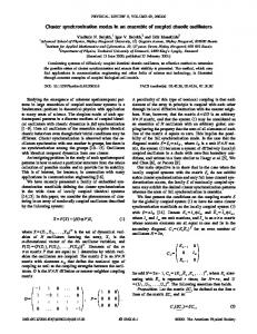
In the present work, we show that the delayed rise of the SE is relying on the excitation of the entire exciton resonance. When exciting only a part of the resonance, the inplane uniformity of the initially excited polarization is broken, and an instantaneous rise of the SE is observed. For excitons in QW’s, the experimental difficulty to measure such an instantaneous rise is to optically excite only a part of the exciton resonance with sufficient temporal resolution, i.e., with a pulse that is wider than the spectral width of the excited exciton distribution. This becomes possible when the exciton resonance is split into separated peaks, which can be achieved by growing QW’s with a growth interrupt on both interfaces. The formation of growth islands larger than the exciton localization length9,10 during the growth interrupt leads to a splitting of the excitonic absorption into distinct lines corresponding to regions of the QW differing in effective thickness by one monolayer 共ML兲. To compare both cases of the initial SE dynamics, we investigate two different samples, grown with or without growth interruption. While the spectral widths of the excited excitonic distributions are similar in both samples, the SE rise is different, instantaneous for the monolayer peak of the growth interrupted sample, and delayed for the continuously grown sample. The two investigated samples are GaAs single quantum wells 共SQW’s兲 grown on GaAs 共100兲 wafers. The first sample 共CG兲 was grown without growth interrupt, and contains a 12 nm thick GaAs well embedded in Al0.3Ga0.7As barriers. In this sample, the surface growth islands are smaller than the exciton Bohr radius, and the segregation as well as the alloy disorder in the barriers introduce a disorder potential with an atomic scale correlation length. The sample shows an asymmetric excitonic absorption line shape 共see Fig. 1兲. Such a line shape is typical for excitons localized by a potential with a correlation length much smaller than the exciton radius.11 The second sample 共GI兲 contains a nominally 11 nm thick GaAs well embedded in AlAs barriers. The growth has been R10 555
©2000 The American Physical Society
RAPID COMMUNICATIONS
R10 556
LANGBEIN, LEOSSON, JENSEN, HVAM, AND ZIMMERMANN
FIG. 1. Optical density of the excitonic resonance in the investigated SQW samples, deduced from the photoluminescence at 30 K lattice temperature. Left: sample GI, a growth interrupted 11 nm GaAs/AlAs well at several positions along the thickness gradient. The labels give the estimated differences in the average well thickness for the different positions. Right: sample CG, a continuously grown 12 nm GaAs/Al0.3Ga0.7As well.
interrupted for 120 s at each interface to enable the formation of larger monolayer islands on the respective surfaces. This results in a splitting of the exciton resonance into so-called monolayer peaks, which are related to excitons localized in QW regions with effective thicknesses differing by integer monolayers. The broadening of each monolayer peak is due to the finite size of the growth islands, leading to varying in-plane quantization energies, and due to an atomic-scale interface roughness formed by segregation during the overgrowth on the surfaces. We have chosen a rather wide GaAs well in order to reduce the spectral width of the monolayer peaks originating from the atomic-scale interface roughness. However, the monolayer splitting is reduced by the same factor, while the in-plane quantization energies are constant, and thus the monolayer peaks are not as well distinguished as for narrower wells. Rotation of the substrate was stopped during the growth of the well in order to achieve a continuous variation in well thickness across the wafer. This allows us to tune the well thickness for the best linewidth. More details about the growth and characterization are given in Ref. 9. In the following experiments we choose the sample position ⫺0.2 ML in Fig. 1. The samples are placed in a helium cryostat at a temperature of 5 K. The exciton resonance is excited by optical pulses from a mode-locked Ti:sapphire laser spectrally shaped to about 1 ps Fourierlimited pulse width. The SE in various directions is spectrally filtered by a monochromator and detected by a synchroscan streak camera with a time resolution of about 3 ps. The angular resolution achieved by the second dimension of the streak camera was adjusted to the speckle size, i.e., to the diffraction limit of the emission from the excited area on the sample.12 The spectral resolution of about 1 meV rejects nonresonant emission, but does not deteriorate the temporal resolution. All presented data were taken with excitation in Brewster angle and detection normal to the sample, through an analyzer parallel to the linear excitation polarization. From the temporally and directionally resolved emission intensity I(t,qជ ), the speckle analysis technique12–15 can deduce the average emission intensity I(t), and the average
PRB 61
FIG. 2. Secondary emission intensity 共open circles兲 and its coherence 共closed squares兲 deduced from the speckle statistics. Left: sample GI for the ⫺0.2 ML position. Right: sample CG. In the insets the intensity spectra of the respective exciting pulse 共dotted line兲 and secondary emission 共solid line兲 are shown.
coherence c⫽I coh/¯I where the average is taken over the scattering directions qជ at fixed time, and I coh is the SE intensity which is coherent to the excitation 共RRS兲. A simple model12 for localized 1s excitons in a SQW is a spatially homogeneous distribution of oscillators with Gaussian distributed, spatially uncorrelated transition frequencies of variance . Each state has the same polarization decay rate due to radiative loss and phonon dephasing, ⌫⫽⌫ rad⫹⌫ phon . For the emitted intensity I(t) after a ␦ -like excitation pulse at t⫽0 one gets12 ¯I 共 t 兲 ⬀e ⫺2⌫ radt 共 1⫺e ⫺ 2 t 2 ⫺2⌫ phont 兲 , c 共 t 兲 ⫽ 共 1⫺e ⫺
2t2
兲 / 共 e 2⌫ phont ⫺e ⫺
2t2
共1兲 兲.
The measured I(t) and c(t) are displayed in Fig. 2 for the two investigated samples. The corresponding SE spectra are shown in the inset together with the exciting laser pulse. The full width at half maximum 共FWHM兲 of the SE spectra are 0.42 共0.4兲 meV for the sample GI 共CG兲, corresponding to ⫺1 ⫽3 ps 共3.3 ps兲. The laser spectra are of 2.3 meV 共1.4 meV兲 FWHM, corresponding to 0.8 ps 共1.3 ps兲 long pulses. Both samples show, after the initial transient, an exponential decay of the secondary emission intensity with 16 ps 共19 ps兲 decay time, and of the emission coherence with 66 ps 共74 ps兲 decay time, respectively. From the decay we deduce according to Eq. 共1兲 a ⌫ rad of 21 eV 共17 eV), and a ⌫ phon of 5 eV 共4.5 eV). Both the lifetime and the dephasing times are thus much longer than the inverse inhomogeneous broadening, which implies that the initial dynamics is dominated by the inhomogeneous broadening and that the initial SE is dominantly RRS. The initial dynamics for both samples is displayed on a linear scale in Fig. 3 together with the response function of the streak camera. The dynamics according to Eq. 共1兲, convoluted with the streak response, is given by the solid lines ( ␣ ⫽1), using the parameters given above. The data for the GI sample show a much faster rise than this calculation, while the data from the CG sample are in full agreement.
RAPID COMMUNICATIONS
PRB 61
INSTANTANEOUS RAYLEIGH SCATTERING FROM . . .
FIG. 3. Initial secondary emission intensity dynamics 共circles兲, compared with the prediction of Eq. 共1兲 共solid兲 and Eq. 共2兲 for ␣ ⫽0.4 共dashed兲, and the instrument response 共dotted兲. Left: sample GI for the ⫺0.2 ML position. Right: sample CG. The inset shows ¯I (t) from Eq. 共2兲 for various values of ␣ and ⌫ rad⫽⌫ phon⫽0.
The dynamics in the GI sample thus do not show the quadratic rise given by the inhomogeneous broadening as predicted by Eq. 共1兲, but a much faster response, indicating an instantaneous contribution to the RRS. To include the influence of growth islands into the model of Eq. 共1兲, we can assign to each exciton a monolayer thickness, where the spatial distribution of the monolayers is random on a length scale of the light wavelength. Only excitons belonging to the selected monolayer are optically excited, and are thus contributing to the SE. With the probability ␣ of an exciton to belong to the excited monolayer, we get ¯I 共 t 兲 ⬀ ␣ e ⫺2⌫ radt 共 1⫺ ␣ e ⫺ 2 t 2 ⫺2⌫ phont 兲 , c 共 t 兲 ⫽ 共 1⫺ ␣ e ⫺
2t2
兲 / 共 e 2⌫ phont ⫺ ␣ e ⫺
2t2
共2兲 兲.
The calculated initial dynamic for different ␣ and neglecting ⌫ rad and ⌫ phon is shown in the inset of Fig. 3. The SE intensity acquires an instantaneous contribution of a fraction 1⫺ ␣ of the total signal. For a small concentration of excited resonances, as it is the case in atomic vapors or for impuritybound excitons in bulk semiconductors, the predicted RRS rise is thus completely instantaneous. For the present case of excitons localized in monolayer islands, typically 2–3 different monolayer thicknesses exist for a given average thickness,9,16,17 which is compatible with ␣ ⬇0.4. In this case, both an instantaneous and a delayed component is expected. The calculation using Eq. 共2兲 convoluted with the streak camera response is given as a dashed line in Fig. 3. It agrees with the data on the GI sample. We thus conclude that the dynamics of the CG sample is well described by the model with a spatially homogeneous distribution of the optically excited excitons. In contrast, the GI sample shows a faster rise, which is instantaneous within our time resolution. We assign this instantaneous RRS contribution to the spatial nonuniformity of the excitons belonging to one monolayer thickness. This behavior is illustrated in Fig. 4. In the CG sample 共upper row兲, the initially excited polarization is constant ( t⫽0), while in the GI sample, only the regions of the selected monolayer thickness are excited, and the polarization has a corresponding spatial pattern, which implies that RRS is present already at t⫽0. For a finite time
R10 557
FIG. 4. Illustration of the spatial dynamics of the macroscopic polarization following excitation of the whole exciton resonance 共top兲 or only one monolayer peak 共bottom兲. The grayscale is linear, and centered at zero. The pictures have been generated from a 64 ⫻64 array of resonances with Gaussian-distributed eigenenergies, excited at t⫽0 by a ␦ pulse. In the case of the GI, the resonances are only active at the positions given by the pattern visible at t ⫽0, for which ␣ ⫽0.5.
after excitation ( t⫽0.5), the initially in-phase excited polarization from the individual localized excitons becomes out of phase, due to their different eigenenergies, which leads to a spatially varying macroscopic polarization. After the initial transient ( t⫽2), the phases of the individual excitons are fully random, and strong SE occurs. This is equivalent in the GI structure, but here, the initial spatial variation is only weakly increasing at later times. The length scale of the monolayer islands is about9 20 nm, significantly lower than the wavelength of the emitted light. The SE is thus emitted isotropically in all directions. Since the growth islands are rather small, typically only one localized exciton state is situated in each island, and the phase of the macroscopic polarization has a common time evolution within one island. On a length scale of 10 nm, the spatial pattern of the macroscopic polarization is thus markedly different for the two investigated structures, which might be important in modelling the long-term RRS dynamics by microscopic models for QW’s with large correlation lengths of the disorder potential.18 In conclusion, we have demonstrated that the initial dynamics of the SE from excitons in QWs can acquire an instantaneous contribution in a situation where the excited exciton polarizability is spatially nonuniform. This is expected not only to be important in the investigated case of a monolayer peak, but also for samples of larger disorder, in which internally excited states of the exciton are mixed into the broadened 1s excitonic resonance. The samples were grown at III-V Nanolab, a joint laboratory between Research Center COM and the Niels Bohr Institute, Copenhagen University. The authors wish to thank Dr. C.B. So” rensen for his assistance with the MBE growth, P. Borri for stimulating discussions, and Tele Danmark R/D for the donation of experimental equipment. This work was supported by the German Science Foundation 共DFG兲 within the ‘‘Schwerpunktprogramm Quantenkoha¨renz in Halbleitern.’’
RAPID COMMUNICATIONS
R10 558 1
LANGBEIN, LEOSSON, JENSEN, HVAM, AND ZIMMERMANN
H. Stolz, D. Schwarze, W. von der Osten, and G. Weimann, Phys. Rev. B 47, 9669 共1993兲. 2 H. Wang, J. Shah, T. Damen, and L. Pfeiffer, Phys. Rev. Lett. 74, 3065 共1995兲. 3 S. Haacke, R. Taylor, R. Zimmermann, I. Bar-Joseph, and B. Deveaud, Phys. Rev. Lett. 78, 2228 共1997兲. 4 D. Birkedal and J. Shah, Phys. Rev. Lett. 81, 2372 共1998兲. 5 S. Haroche, in High Resolution Laser Spectroscopy, Vol. 13 of Topics in Applied Physics 共Springer, Berlin, 1976兲, pp. 253– 313. 6 R. Zimmermann, Nuovo Cimento D 17D, 1801 共1995兲. 7 D. S. Citrin, Phys. Rev. B 54, 14 572 共1996兲. 8 S. Haacke, G. Hayes, R. A. Taylor, B. Deveaud, R. Zimmermann, and I. Bar-Joseph, Phys. Status Solidi B 204, 35 共1997兲. 9 K. Leosson, J. R. Jensen, W. Langbein, and J. M. Hvam, Phys. Rev. B 61, 10 322 共2000兲. 10 H. Castella and J. W. Wilkins, Phys. Rev. B 58, 16 186 共1998兲.
PRB 61
R. Zimmermann and E. Runge, J. Lumin. 60-61, 320 共1994兲. W. Langbein, J. M. Hvam, and R. Zimmermann, Phys. Rev. Lett. 82, 1040 共1999兲. 13 W. Langbein and J. M. Hvam, in Advances in Solid State Physics, edited by B. Kramer 共Vieweg, Braunschweig, 1999兲, Vol. 39, pp. 463–472. 14 E. Runge and R. Zimmermann, in Advances in Solid-State Physics, edited by B. Kramer 共Vieweg, Braunschweig, 1999兲, Vol. 39, pp. 423–432. 15 W. Langbein and J. M. Hvam, Phys. Status Solidi A. 共to be published兲. 16 D. Gammon, B. V. Shanabrook, and D. S. Katzer, Phys. Rev. Lett. 67, 1547 共1991兲. 17 R. F. Kopf, E. F. Schubert, T. D. Harris, and R. S. Becker, Appl. Phys. Lett. 58, 631 共1991兲. 18 V. Savona, S. Haacke, and B. Deveaud, Phys. Rev. Lett. 84, 183 共2000兲. 11 12