using standard syste - Purdue Math - Purdue University

PHYSICAL REVIEW E

VOLUME 62, NUMBER 1

JULY 2000

Critical transitions in colliding cascades A. Gabrielov Department of Earth and Atmospheric Sciences and Department of Mathematics, Purdue University, West Lafayette, Indiana 47907-1395

V. Keilis-Borok International Institute of Earthquake Prediction Theory and Mathematical Geophysics, Russian Academy of Sciences, Warshavskoe shosse, 79, korpos 2, 113556, Moscow, Russia and Department of Earth and Space Sciences and Institute of Geophysics and Planetary Physics, University of California, Los Angeles, California 90095-1567

I. Zaliapin International Institute of Earthquake Prediction Theory and Mathematical Geophysics, Russian Academy of Sciences, Warshavskoe shosse, 79, korpos 2, 113556, Moscow, Russia

W. I. Newman Department of Earth and Space Sciences, Department of Physics and Astronomy, and Department of Mathematics, University of California, Los Angeles, California 90095-1567 共Received 9 November 1999兲 We consider here the interaction of direct and inverse cascades in a hierarchical nonlinear system that is continuously loaded by external forces. The load is applied to the largest element and is transferred down the hierarchy to consecutively smaller elements, thereby forming a direct cascade. The elements of the system fail 共i.e., break down兲 under the load. The smallest elements fail first. The failures gradually expand up the hierarchy to the larger elements, thus forming an inverse cascade. Eventually the failures heal, ensuring that the system will function indefinitely. The direct and inverse cascades collide and interact. Loading triggers the failures, while failures release and redistribute the load. Notwithstanding its relative simplicity, this model reproduces the major dynamical features observed in seismicity, including the seismic cycle, intermittence of seismic regime, power-law energy distribution, clustering in space and time, long-range correlations, and a set of seismicity patterns premonitory to a strong earthquake. In this context, the hierarchical structure of the model crudely imitates a system of tectonic blocks spread by a network of faults 共note that the behavior of such a network is different from that of a single fault兲. Loading mimics the impact of tectonic forces, and failures simulate earthquakes. The model exhibits three basic types of premonitory pattern reflecting seismic activity, clustering of earthquakes in space and time, and the range of correlation between the earthquakes. The colliding-cascade model seemingly exhibits regularities that are common in a wide class of complex hierarchical systems, not necessarily Earth specific. PACS number共s兲: 05.65.⫹b, 91.30.Px, 91.30.Dk, 64.60.Ht

I. INTRODUCTION

We synthesize here three phenomena that play an important role in many complex systems. First, the system has a hierarchical structure, with the smallest elements merging in turn to form larger and larger ones, the largest element being the entire system. Second, the system is continuously loaded or driven by external sources. Finally, the elements of the system fail 共break down兲 under the load, causing redistribution of the load throughout the system. Eventually the failed elements ‘‘heal’’ and regain their structural integrity, thereby facilitating the continuous operation of the system. The load is transferred from the top of the hierarchy to the bottom, thus forming a direct cascade from the largest to the smallest scales. Failures are initiated at the lowest level of the hierarchy or tree, and gradually propagate upward, thereby forming an inverse cascade. The interaction of direct and inverse cascades establishes the dynamics of the system. Direct cascades are well known, for example, in the theory of three-dimensional turbulent flow where energy 1063-651X/2000/62共1兲/237共13兲/$15.00

PRE 62

and/or momentum is transferred from large eddies to small ones, eventually dissipating through viscosity 关1兴. Another example is plate tectonics—the influence of mantle convection is transferred to consecutively smaller structures 关2兴. Examples of inverse cascades 关3兴 include the escalating sequence of earthquakes; avalanches in rock, sand, and snow; the consecutive coalescence of fractures in a solid body; forest fires and epidemics; the clustering of animals into flocks, herds, schools, and so on; and chain reactions in physics, chemistry, and economics. In many systems both direct and inverse cascades coexist and interact. Loading increases instability and causes an inverse cascade of failures, while failures release and redirect loading. In this study we model such an interaction. The hierarchical structure of the model imitates the active lithosphere, composed of a hierarchy of volumes 共‘‘blocks’’兲 separated by faults. Loading in the model imitates the influence of tectonic forces, while failures imitate earthquakes. We focus here on the collective behavior of multiscale failures, which correspond to the seismicity of a fault net237

©2000 The American Physical Society

238

GABRIELOV, KEILIS-BOROK, ZALIAPIN, AND NEWMAN

FIG. 1. Structure of the three-branched or ternary tree model. Figure shows four highest levels of the seven-level tree, used in simulation.

work, and not on the dynamics of a single failure. Moreover, we explore the major robust features of the behavior of colliding cascades. Accordingly, as is usually the case in such models, we employ the basic condition of failure specified in Sec. II D below. Heuristic or empirical constraints are derived from studies of seismicity. We make the model as simple as we can, providing a skeletal representation of a real lithosphere with its immense complexity. Nevertheless, the model reproduces the major regularities in the observed dynamics of seismicity, namely, the seismic cycle, intermittency in the seismic regime, power-law energy distribution, clustering in space and time, long-range spatial correlations, and a wide variety of seismicity patterns premonitory to a strong earthquake. We consider here three basic types of premonitory pattern. Two patterns of the first type reflect the rise of seismic activity. The pattern of the second type reflects the rise in the clustering of earthquakes in space and time; and two patterns of the third type mirror the rise in the correlation distance between the earthquakes. Each pattern was defined separately for different magnitude ranges. Although the model of colliding cascades reproduces so well the major features of earthquake sequences, the design of the model is not specific to seismicity, or even to the more general phenomenon of multiple fracturing in solids. Our model probably exhibits regularities that are common to a wide class of complex hierarchical systems. Turcotte et al. 关4兴 provide a theoretical basis for such universality, outlining the connection between seismicity and other processes with power-law scaling, such as those studied in statistical physics. II. COLLIDING-CASCADE MODEL

We begin by providing an overview of the structure and dynamics of the simple dynamical system that we are constructing. We then proceed to describe the processes of loading, failure, and healing as well as the governing differential equations. Finally, we describe a synthetic sequence of failures 共‘‘earthquakes’’兲 and demonstrate how it is generated by the interaction of direct and inverse cascades.

PRE 62

ments of the system, and each element has its own index, consisting of two numbers i⫽(m 兩 g). Here, m is the level where an element is situated and is enumerated from the bottom to the top of the hierarchy. The second integer g identifies the position of an element within its level m, count¯ ¯ ing from left to right, namely, from 1 to 3 m ⫺m , where m identifies the top level in the hierarchy. Indexing of elements is illustrated in Fig. 1. It is convenient to describe the taxonomy of this system using the imagery of a family tree. The ¯ 兩 1) has three ‘‘children’’—the elements (m ¯ top element (m ¯ ⫺1 兩 2), and (m ¯ ⫺1 兩 3). They are referred to as ⫺1 兩 1), (m ¯ 兩 1) identifies their ‘‘par‘‘siblings’’ while the element (m ¯ ⫺2 兩 4), (m ¯ ⫺2 兩 5), and ent.’’ For example, the elements (m ¯ ¯ ⫺1 兩 2) (m ⫺2 兩 6) are the children of the parent element (m and the siblings of each other. Conceptually, this structure is similar to that of a wavelet, where the complementary dimensions, crudely, the position and the 共logarithm兲 of the wavelength, have a direct physical meaning and significance. B. Dynamics

The behavior of an arbitrary element i is described by two functions, namely, a continuous positive-valued function ␴ i (t) and a Boolean function f i (t). We think of ␴ i (t) as the ‘‘load’’ supported by an element and of f i (t) as its ‘‘state.’’ An element i is ‘‘whole’’ or intact when f i (t)⫽0, and ‘‘broken’’ or failed when f i (t)⫽1. The direct cascade of loading is described by the set of functions 兵 ␴ i (t) 其 while the inverse cascade of fracturing is described by the set of functions 兵 f i (t) 其 . The dynamics of the system is described by interaction of direct and inverse cascades. The functions ␴ i (t) satisfy a system of ordinary differential equations with the right sides depending upon the functions 兵 f j (t) 其 . The functions f i (t) change their values according to certain logical rules or conditions that depend upon ␴ i (t) and 兵 f j (t) 其 . C. Loading

¯ 兩 1), First, we introduce equations for the top element (m namely.

␴˙ top共 t 兲 ⫽

再

v⫺

␤ ␴ top共 t 兲关 ␪ ⫺ ␴ top共 t 兲兴

v ⫺ ␣ ␴ top共 t 兲

if

f top共 t 兲 ⫽0

if

f top共 t 兲 ⫽1,

共2.1兲

where v ⬎0, ␤ ⬎0, ␪ ⬎0, and ␣ ⬎0. Here v is a constant describing the application of the load to the top element of the system. Note that, in the present realization of the model, this is the only method for introducing a load into the system. The load is transferred in this ternary model to the three ¯ ⫺1 兩 1), (m ¯ ⫺1 兩 2), and (m ¯ ⫺1 兩 3). The rate of elements (m load outflow in Eq. 共2.1兲 depends on the state of the top element. If this element is whole, i.e., f top(t)⫽0, then the rate is equal to

A. Structure

␤ ␴ top共 t 兲 , 关 ␪ ⫺ ␴ top共 t 兲兴

We consider a dynamical system acting on the ternary tree shown in Fig. 1. Nodes of the tree are called the ele-

where ␤ is a constant. If this element is broken, i.e., f top(t)

PRE 62

CRITICAL TRANSITIONS IN COLLIDING CASCADES

⫽1, then the rate is proportional to the load accumulated by the element at that instant of time. In the stationary or steady state case, when the time derivatives in Eqs. 共2.1兲 vanish, we have w ␴ top,ss ⬅

␪v v⫹␤

共2.2兲

for a whole element, and b ␴ top,ss ⬅

v

共2.3兲

␣

¯ 兩 1) tends to for a broken one. The load of the top element (m approach the values 共2.2兲 or 共2.3兲, depending on the state of the element. It is clear from Eq. 共2.1兲 that the load applied to the top element in the whole state can never exceed ␪ . We shall call ␪ a ‘‘critical threshold’’ for the load. ¯ 兩 1) are constructed in a Equations for ␴ i (t) for all i⫽(m ¯ manner analogous to those for (m 兩 1). The only difference is ¯ 兩 1) receives a load not only from its that each element i⫽(m parent but from its siblings as well. Furthermore, the rate of load transfer depends on the load accumulated by the parent and the siblings at that time, namely,

␴˙ i 共 t 兲 ⫽U i 共 t 兲 ⫺W i 共 t 兲 . Here

W i共 t 兲 ⫽

再

共2.4兲

b ␴ i,ss ⬅

v

␣

共2.6兲

for a broken one. Note that these steady state solutions are the same as those for the top element via Eqs. 共2.2兲 and 共2.3兲. We assume that at time t⫽0 all elements are intact, i.e., f i (0)⫽0, and support no load, i.e., ␴ i (0)⫽0. As given by Eqs. 共2.4兲, the load is added to the hierarchical system through the top element and is subsequently redistributed among all other elements in the tree. Since all dynamical equations are symmetric with respect to the siblings’ indices (i,s1,s2), all of the elements on any level retain the same load until at least one element fails. D. Failure

¯ 兩 1) fails when the following conA whole element i⫽(m dition is satisfied:

␴ i 共 t 兲 ⭓ ␪ q ⫺[ f c1 (t)⫹ f c2 (t)⫹ f c3 (t)] ⫻s ⫺[ f s1 (t)⫹ f s2 (t)] , q⭓1,

s⭓1.

共2.7兲

Here, the subindices c1, c2, and c3 refer to the three children of the ith element while s1 and s2 refer to its two siblings. The exponents of q and of s indicate the number of broken children and siblings, respectively. If all children and siblings of the ith element are intact, then this condition reduces to

␴ i共 t 兲 ⭓ ␪ .

␤ ␴ i共 t 兲关 ␪ ⫺ ␴ i 共 t 兲兴

if

f i 共 t 兲 ⫽0

␣ ␴ i共 t 兲

if

f i 共 t 兲 ⫽1

If some of the siblings or children are broken, the ith element is weakened, that is, the threshold for failure is reduced. The parameters q and s in Eqs. 共2.7兲 quantitatively determine this weakening. Equation 共2.7兲 describing the top element reduces to

and U i 共 t 兲 ⫽CW p 共 t 兲 ⫹

239

1⫺C 1⫺C W s1 共 t 兲 ⫹ W s2 共 t 兲 , 2 2

0⭐C⭐1.

The subindex p refers to the parent of the ith element, while subindices s1 and s2 refer to its two siblings. In order to maintain parallelism, we define for the top element

再

␤ ␴ top共 t 兲 ␪ W top共 t 兲 ⫽ 关 ⫺ ␴ top共 t 兲兴 ␣ ␴ top共 t 兲

if

f top共 t 兲 ⫽0

if

f top共 t 兲 ⫽1,

U top共 t 兲 ⫽ v . With this notation, the loading is described by the system 共2.4兲. As before, the load supported by an intact element can never exceed the critical threshold ␪ . In the stationary case, when the time derivatives in Eqs. 共2.4兲 vanish, we have the steady state solutions w ␴ i,ss ⬅

for a whole element i, and

␪v v⫹␤

共2.5兲

␴ top共 t 兲 ⭓ ␪ q ⫺[ f c1 (t)⫹ f c2 (t)⫹ f c3 (t)] due to the absence of siblings. As we have mentioned above, the load applied to an intact element can never exceed ␪ . Therefore, an element cannot fail until at least one of its siblings or children fails. Accordingly, the failures propagate upward and thereby form an inverse cascade. At the bottom level of the tree where the elements have no children, we introduce random failures with a rate proportional to the intensity of the direct cascade. This mimics ‘‘juvenile cracking’’ in earthquake phenomenology. Let t s be the time when the load of an element rises close to the staw ⫺ ⑀ for ⑀ small and positive. This tionary value, ␴ i (t)⭓ ␴ i,ss element fails at a later time t s ⫹ ␹ , where ␹ is a random variable, distributed exponentially with a decay time ␭. This randomness ensures that the dynamics of our model shows a degree of inhomogeneity in spite of the above mentioned symmetry. E. Healing

In order to ensure the perpetual operation of our system, we introduce the effect of ‘‘healing,’’ i.e., the restoration to an unbroken state of a previously broken element. Otherwise the system will cease to function once all elements have


240

PRE 62

failed. We assume that a broken element heals when the following two conditions hold during the ensuing exponentially distributed time interval with a decay time L. At least n children of the ith element are intact, and

␴ i 共 t 兲 ⬍ ␪ q ⫺[ f c1 (t)⫹ f c2 (t)⫹ f c3 (t)] s ⫺[ f s1 (t)⫹ f s2 (t)] .

共2.8兲

Finally, at the bottom level we replace the latter by

␴ i共 t 兲 ⬍ ␪ .

共2.9兲

Having formulated our model, we now provide it in dimensionless form. F. Dimensionless equations

Equations 共2.4兲 contain values of ␴ i (t) measured in units 关 u 兴 , and time measured in units 关 t 兴 . Meanwhile, the variables v and ␤ are measured in units 关 u/t 兴 , variable ␪ in 关 u 兴 , ␣ in 关 t ⫺1 兴 , and ␭ and L in 关 t 兴 . We now define a time scale t 0 ⫽ ␪ / v . Let us introduce the following dimensionless variables:

␶ ⬅t/t 0 ,

˜␴ i 共 ␶ 兲 ⬅

␴ i共 t 兲 , ␪

FIG. 2. Synthetic earthquake sequence. The complete sequence is shown on the top panel followed by exploded views in the following three panels. Note that all times given, in this and subsequent figures, are in dimensionless units.

共 t k ,m k ,g k 兲 ,

and dimensionless parameters

␥⬅␤/v, ˜␣ ⬅

␣␪ v

.

We then obtain the dimensionless equations ˜␴˙ i 共 ␶ 兲 ⫽U ˜ i 共 ␶ 兲 ⫺W ˜ i共 ␶ 兲 . Here

˜ i共 ␶ 兲 ⫽ W

再

␥ ˜␴ i 共 ␶ 兲 ␴ i 共 ␶ 兲兴关 1⫺ ˜

if

f i 共 ␶ 兲 ⫽0

˜␣ ˜␴ i 共 ␶ 兲 ,

if

f i 共 ␶ 兲 ⫽1,

˜ i 共 ␶ 兲 ⫽CW ˜ p共 ␶ 兲 ⫹ U

共2.10兲

1⫺C 1⫺C ˜ s1 共 ␶ 兲 ⫹ ˜ s2 共 ␶ 兲 W W 2 2 ¯ 兩1 兲, i⫽ 共 m

˜ i 共 ␶ 兲 ⫽1, U

¯ 兩1 兲. i⫽ 共 m

As before, the subindex p refers to the parent of the ith element, while the subindices s1,s2 refer to the two siblings of ith element. G. Sequence of failures

The colliding-cascade model determines for each element both the load ␴ i (t) and the state f i (t)—whether the element is broken or whole. In many relevant processes, including seismicity, the data for failure events are especially complete since it is easier to both measure and catalog the failures than the load. We represent the sequence of failures as

t k ⭐t k⫹1 .

k⫽1,2, . . . ,

共2.11兲

Here, t k is the time of failure for an element, whereas m k and g k indicate its position within the model 共see Fig. 1兲. The usual basic representation of an observed earthquake sequence is very similar to Eq. 共2.11兲, where the vector g k constitutes the coordinates of the hypocenter, i.e., the actual point of origin of an earthquake event 共the epicenter is its projection on the Earth’s surface兲. Often overlooked, however, is the fact that the region of rupture, which we will later call L, is 101 –102 km in extent for earthquakes with magnitudes between 7 and 8. Earthquakes are not point source events. An earthquake starts with a localized rupture that then spreads on a complex surface of finite dimensions and has distinctly different near-field, intermediate zone, and farfield effects. Strictly speaking, this model has no three-dimensional space of hypocenters, but we regard g to be a coarse analog of the hypocenter, since it identifies the position of a failed element in relation to other ones 共see Fig. 1兲. Finally, we regard the value m in synthetic earthquake sequences as an analog of the earthquake magnitude—the latter is a logarithmic measure of energy released by an earthquake. An example of the sequence generated by the collidingcascades model is shown in Fig. 2. It was computed using the numerical parameters provided in Table I. The entire sequence is shown in the top panel, followed by a sequence of exploded views. Each event is formed by simultaneous failure of one or more elements. In a case when several elements fail at the same time, only the events at the highest TABLE I. Values of parameters used in computations.

␥ 0.2

˜␣

C

q

s

⑀

␭

L

n

27.2

0.9

1.096

1.03

0.1

3.0

3.4

2

PRE 62


241

duces the basic regular features of real seismicity. III. HEURISTIC CONSTRAINTS: REGULARITIES IN OBSERVED SEISMICITY

Real earthquake sequences exhibit a high degree of complexity but, upon averaging, manifest a remarkable degree of regularity—such is the usual case in complex systems. We summarize these features in this section and compare them with synthetic seismicity in Secs. IV and V. A. Seismic cycle

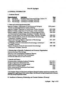
The level of seismic activity or seismicity in an area goes through three different phases 关5兴. First, there is a‘‘preseismic’’ rise culminating in one or several major earthquakes. This is followed by a period of ‘‘postseismic’’ activity, which gradually declines with time. Finally, there emerges a long period of relatively low activity that ultimately returns to another rise, and so on. Such transitions take place in different time and space scales. The characteristic time interval between the strongest earthquakes in active regions, such as southern California, is of the order of 101 –102 years. Usually, however, there is no real periodicity. Observed intervals between major earthquakes depart considerably from the mean, and the character of each phase in the ‘‘seismic cycle’’ varies strongly from case to case. In different epochs, seismic cycles may culminate in earthquakes of different magnitude. Generally, a seismic regime exhibits large intermittency. FIG. 3. Cascades in the five highest levels of the model. Figure portrays the case history of a cycle. Shading is employed to describe proximity in time to failure—the darker the shade, the closer an element to the critical threshold ␪ . Black dots identify broken elements. The time remaining to the major event is indicated at each frame.

level in the hierarchy are indicated. The vertical scale shows their maximum level, referred to as a ‘‘magnitude’’ m. Figure 3 shows the interaction between direct and inverse cascades prior to a major failure, i.e., m⫽7, and following its aftermath. Until some time 共i.e., the initiation of rupture兲, we can see only a direct cascade moving downward 共a兲. After a while 共b兲, the cascade has reached the lowest level and triggers the inverse cascade that is shown in 共c兲. The inverse cascade triggers the rupture that in turn triggers secondary direct cascades. Panel 共d兲 describes the instant when inverse cascade has reached the second-highest level, namely, level, 6. The elements with the darkest shading identify a secondary direct cascade, triggered by a failure at that level. Meanwhile, the secondary direct cascade is evolving 共e兲 and triggers an aftershock at level 5 共the darkest broken element兲. Panel 共f兲 demonstrates another inverse cascade that is initiated in the right hand branch of the model. It triggered instantaneous failure that propagated to top level. These failures are connected in the figure. Panel 共g兲 shows that yet another secondary direct cascade has started. Finally, the inverse cascade is weakening 共h兲. Healing prevails until the subsequent direct cascade reaches level 1. In subsequent sections, we investigate whether synthetic seismicity generated by the colliding-cascade model repro-

B. Power-law energy distribution

Otherwise known as the Gutenberg-Richter law 关6–11兴, the energy distribution of earthquakes in a fault system may be approximately described as log10 N 共 m 兲 ⫽a⫺bm.

共3.1兲

Here, N(m) is the average annual number of earthquakes with magnitude above m in a specified spatial region. This law is valid for sufficiently large fault systems and time intervals and for a certain magnitude range 关 m 1 ,m 2 兴关8兴. It is important to note that it does not describe the frequency of events on a small-scale, individual fault. Typically, b⬇1, not changing much with variation of the geometry of the fault system, the local tectonics, and so on, thereby hinting at a universal mechanism for the dynamics of seismicity. The power-law energy distribution 共3.1兲 is at the heart of many models of seismicity. It is noteworthy, therefore, that Eq. 共3.1兲 is only an approximation to real seismicity. The most frequently observed deviations from Eq. 共3.1兲 that are not attributable to inaccurate observations are summarized below. 共a兲 log10 N(m) bends over or changes slope at the largest magnitudes 关6,8兴. In the case of a downward bend, the Kolmogoroff log-normal relation 关12兴, which describes the distribution of the size of the rocks in a fractured massive region, sometimes happens to fit the earthquake energy distribution better than Eq. 共3.1兲. In some cases, however, there is an upward bend 关13兴, or the values of N(m) for the largest m are scattered above the power-law approximation

242


共3.1兲. Such magnitudes are often attributed to what is sometimes called a ‘‘characteristic earthquake,’’ an event having the maximum possible size in the region considered 关7,14兴. 共b兲 log10 N(m) may be represented by a collection of overlapping power laws with statistically significant differences in the slope b of the different segments 关8,15兴. 共This refers to the whole magnitude range, as well as to what was described above for its ends.兲共c兲 The shape and parameters of the energy distribution change with time. This includes two kinds of changes premonitory to a major earthquake. 共1兲 The upward bend of distribution for relatively large m 关13,16兴; it reflects premonitory increase of seismic activity. 共2兲 A possible increase in the b value for smaller magnitudes. In 关15兴 such changes are found both in the observed seismicity and in fracturing of steel samples. 共d兲 For the physical interpretation of the GutenbergRichter law 共3.1兲 its multiscale nature is primal 关10,8兴. Statistics of earthquakes with magnitude m have to be established in spatial regions of linear dimension much larger than L(m), the characteristic dimension of the earthquake source. Accordingly, the parameters a and b have to be determined for increasingly larger areas, when larger magnitude ranges are considered. The above deviations from the power law 共3.1兲 depend on the spatial scale considered. For larger regions some of them may disappear. We now return to other forms of regularity observed in seismicity.

C. Clustering

Earthquakes are observed to cluster in both space and time 关9,17,18兴. A typical cluster is a main shock, namely, the earthquake, followed by a string of weaker shocks, called aftershocks. Some earthquakes are also preceded by foreshocks of a smaller magnitude. Typically, about 30% of main shocks have foreshocks. The number of foreshocks is usually small. Clusters of another kind, known as ‘‘swarms,’’ are formed by main shocks of comparable magnitude that occur in proximity 共in both space and time兲 to each other, with their own overlapping sets of aftershocks and foreshocks 关19兴. D. Premonitory seismicity patterns

Often, a strong earthquake in a region is preceded by a set of unusual patterns of seismicity 共关20–22兴 and references therein兲. This anticipatory behavior was summarized by Keilis-Borok 关23兴 as follows. Typically, a few years in advance of a strong earthquake, a sequence of seismic events in a medium magnitude range becomes increasingly intense and irregular. These events become more clustered in both space and time, and their correlation distance probably increases. All of these phenomena may be caused by an increased response of the lithosphere to excitation. The scaling of these phenomena depends on the scale of the ‘‘strong’’ earthquake they foretell. Let M be its magnitude, and L(M ) be the linear size of its source. These phenomena are defined, then, in the magnitude range down to about M ⫺4, and in a region of linear dimension of 5L –10L. They precede a strong earthquake by a few years.

PRE 62

FIG. 4. Composite catalog. All cycles are combined, with each major event placed at time t⫽0.

Such premonitory phenomena, formally defined, have been used in algorithmic earthquake prediction—see 关22,23兴 and references cited therein. We apply here the same definitions of premonitory behavior to synthetic seismicity generated by our model. In addition, we consider accelerating Benioff stress release—a precursor described in 关24–27兴. It consists of power-law escalation of seismicity possibly including an accelerating and, possibly, log-periodic oscillatory component. IV. SYNTHETIC SEISMICITY: SEISMIC CYCLE, ENERGY DISTRIBUTION, AND CLUSTERING

Here, and in the next section, we demonstrate that the colliding-cascade model reproduces many of the regular features of observed seismicity, described in the previous section. The major advantage provided by our synthetic sequence is the relative simplicity of its temporal structure. That facilitates the establishment of connections between different forms of regularity, and the possible identification of yet undiscovered regularities or patterns, which can then be validated by analysis of observations. Seismic cycles. About half of the time, the sequence shown in Fig. 2 consists of well-separated cycles, culminating in a ‘‘major event’’ of magnitude 7. There is clear intermittency in the seismic regime—seismicity is very different during the time interval 900–2200 time units—the magnitudes there do not exceed 6, and separation of the record into individual time cycles is not clear. Possibly, this interval includes shorter seismic cycles culminating in earthquakes with m⫽6. Such seismic intermittency is also typical in real seismicity. A composite portrait of the seismic cycle is shown in Fig. 4. All seismic cycles are superimposed in this figure with each major event centered at the same time origin, i.e., t⫽0. The top panel shows all earthquakes, in a linear time scale, while the bottom panel shows mainshocks and aftershocks in logarithmic time scale. Energy distribution. Figure 5 shows the energy distribution in our synthetic earthquake sequence. We see that it fits well the Gutenberg-Richter law 共3.1兲 without strong deviations. Clustering. We have identified the aftershocks by the same method as is used in analysis of observations; it is

PRE 62


243

FIG. 5. Energy distribution function, log10 N⫽a⫺bm where N is the number of events with magnitude m. Note that the magnitude is given discrete integer values from 1 to 7.

described in the Appendix. Statistics of aftershocks are shown in Fig. 5. We see here the features in common with real seismicity—aftershocks constitute about half of the earthquake events, and the b parameter of the GutenbergRichter law for aftershocks is slightly higher than for main shocks. V. SYNTHETIC SEISMICITY: PREMONITORY SEISMICITY PATTERNS

Here we apply to the analysis of earthquake precursors an approach known as ‘‘pattern recognition of infrequent events.’’ It was developed by Gelfand co-workers over two decades ago for the study of rare phenomena of highly complex origin, a situation where classical statistical methods are inapplicable. The methodology of pattern recognition is very robust and its essence will be clear from the way synthetic data are analyzed here. In our problem, the goal of pattern recognition is the identification of behavior that almost always occurs before a main shock, yet almost never occurs otherwise. A more detailed description can be found in 关28兴. In this approach to the search for earthquake precursors, we conventionally divide the time period considered into intervals of three kinds, which are designated by the symbols

D, N, and X. Figure 6 illustrates this division. An interval D precedes a major earthquake—that letter is chosen to mnemonically represent ‘‘danger.’’ An interval X follows it and is characterized by post-major-earthquake activity, including waning aftershock sequences. The latter have a characteristically inverse time rate of occurrence sometimes known as Omori’s law. The rest of the time between the major earthquakes comprises the 共null兲 intervals N; thus, they are distanced from major earthquakes. This division of time allows

FIG. 6. Division of time into three kinds of periods: interval D—less than 20 time units before a major event (m⫽7); interval X—within 20 time units after a major event; and interval N—all other time intervals, except empty ones. Premonitory phenomena are considered in the last D 0 time units of each interval D.

244


us to explore precursors by the pattern recognition approach. A precursor is recognized if it seems to emerge in the intervals D more frequently in a statistically significant way than in intervals N. 共Ideal precursors emerging only in the intervals D have yet to be found.兲 The application of such an approach to the observed seismicity is described in 关23,29兴 and references therein. Several precursors considered in the next section have been identified using the above condition. Now, we explore whether they exist in our synthetic seismicity. First, we eliminate the intervals X from the search for precursors, since these intervals are dominated by specific features of post-major-earthquake activity, even if we exclude aftershocks. 共These intervals, however, are considered separately for prediction of a second strong earthquake, in a pair 关30兴. This problem is beyond the scope of the present study.兲 The exact duration of D intervals is not known a priori. To ensure sufficient separation between intervals D and N, we consider in each interval D only the final D 0 time units preceding a major event. Empty intervals between the cycles are disregarded. We assume the duration 20 time units for the intervals D and X, independently of what precursor is explored. D 0 is chosen to be 3 or 5 time units, depending on the precursor. A. Statistically significant precursors validated by prediction of real earthquakes

The precursors considered here have been identified by the analysis of observations of real earthquakes, with the pattern recognition approach described above 共关21,22兴 and references therein兲. They are defined on the sequence of main shocks. Elimination of aftershocks from the sequence is necessary for the following reason. On average, the total number of aftershocks grows with the magnitude of the main shock. Therefore, unless aftershocks are eliminated, the relatively strong main shocks would be represented in premonitory patterns twice—by themselves and by their aftershocks. However, for each main shock, we retain the number of its aftershocks; these numbers are used in the definition of premonitory clustering. 1. Clustering

We consider as a measure of clustering the function B m (t k 兩 ␶ ) which identifies the number of aftershocks within a time interval ␶ following a main shock 关31–33兴. Here, m is the magnitude of the main shock, while k identifies its position in the sequence of main shocks. Thus, t 1 denotes the time of the first main shock, t 2 the second, and so on. In earthquake prediction studies, B m is assessed over a very short time interval, namely, ␶ ⫽2 days, while the ensuing aftershock sequence may last a year or more. The application of this measure to observed seismicity is described in detail in 关31,34兴. In our analysis of synthetic events, we assume ␶ ⫽0.05 time units. Let P D (B m ) be the density distribution of the values of B m taken collectively from all intervals D. Similarly, P N (B m ) is the density distribution corresponding with the intervals N. Precursory behavior in the variable B m is characterized, according to a familiar Bayesian approach, by the

PRE 62

difference of these densities, namely, ⌬ 共 B m 兲 ⫽ P D共 B m 兲 ⫺ P N共 B m 兲 . If large values of B m preferentially occur prior to a major event, then the function ⌬ should be positive for these values of B m , and negative for smaller ones. To make our analysis robust, we divide all the values of B into three groups, namely, ‘‘small,’’ ‘‘medium,’’ and ‘‘large.’’ They are separated by the percentiles of the levels 33.3% and 66.6%. In other words, this division is made using the condition that each group contains equal numbers of events and, therefore, equal numbers of values B. This is done for the intervals D and N taken together so that a priori knowledge of major events is not used in discretization of the values of B. The functions ⌬(B 6 ) and ⌬(B 5 ), thus discretized, are shown in panels 共a兲 and 共b兲 of Fig. 7 . The last D 0 ⫽5 time units are considered in the intervals D. Note that ⌬ is given as a percentage. We see clearly that the generation of aftershocks tends to be larger in D. Similar results were obtained for m⫽2, 3, and 4. 2. Premonitory rise of seismic activity

Following 关29,35兴 and references therein, we consider two functions reflecting the premonitory rise of seismic activity. These functions are N m (t 兩 s), defined as the number of main shocks with magnitude m, and ⌺ m共 t 兩 s 兲 ⫽

兺 S k共 t 兩 s 兲 .

Here, S k is the area of rupture in the earthquake source, where k again is its number in the sequence of main shocks. Summation is taken over all the main shocks with magnitude less than or equal to m. In the analysis of real observations, this area is crudely estimated from the earthquake magni¯ tude. For synthetic seismicity, we assume that S i ⫽3 m⫺m , ¯ is the index of the top level; this value is proporwhere m tional to the number of elements at the lowest or first level that are the offspring of the element on level m 共Fig. 1兲. The ¯ 兩 1), is unity. contribution of the top element, namely, (m Both functions N m (t 兩 s) and ⌺ m (t 兩 s) are counted in a sliding time window (t⫺s,t), where s⫽2. Note that their values are attributed to the end of this window so that information from the future is not used. Panels 共c兲–共e兲 of Fig. 7 display the functions ⌬(N 1 ), ⌬(N 2 ), and ⌬(⌺ 6 ). The final D 0 ⫽3 time units are considered in the intervals D. We clearly see that each measure tends to be larger in D. Similar results were obtained for N m , m⫽3,4,5, and for ⌺ m with m varying from 2 to 5. B. A precursor explored by retrospective analysis of observations: ‘‘Accelerated Benioff strain release’’

In the studies by Bufe and Varnes, 关24兴, Sornette and Sammis 关25兴, Newman et al. 关26兴, and Johansen et al. 关27兴共see also references therein兲, premonitory escalation of seismicity is represented by the empirically based function

⑀ 共 t 兲 ⫽ ⑀ 0 ⫺B 共 t f ⫺t 兲 ␣ . Here, ⑀ is the cumulative Benioff stress release

PRE 62


245

FIG. 7. Premonitory phenomena depicted by the difference of distributions within intervals D and N. ⌬(F) is the difference between distributions of values of premonitory function F(t) within intervals D and N. Concentration of high values of the function F(t) within the intervals D is depicted by positive differences ⌬(F), which can be 共a兲 ⌬(B 6 ); 共b兲 ⌬(B 5 ); 共c兲 ⌬(N 1 ); 共d兲 ⌬(N 2 ); 共e兲 ⌬(⌺ 6 ); or 共f兲 ⌬(R).

⑀ ⫽ 兺 E 1/2 k as a function of time over the interval (t 0 ,t), E k is earthquake energy estimated from the magnitude with the summation taken over all earthquakes in the region without the elimination of aftershocks, and t f is the actual time of a strong earthquake. Figure 8 demonstrates this phenomenon on the composite seismic cycle shown in Fig. 4. We see that ⑀ indeed is rising steeply starting at about 10 time units before the major earthquake. Panel 共a兲 in Fig. 8 gives the usual representation of that function while panel 共b兲 shows that, during a time interval from ⫺5 to ⫺1 time units, the function ⑀ is rising according to a power law, with ␣ ⫽0.4. However, unlike the reported real observations, the growth of synthetic seismicity terminates about 0.5 time units before a major earthquake. C. Potential precursors not yet identified in observations

We consider the premonitory increase in the range of spatial correlation between the earthquakes. Qualitatively, this

phenomenon was hypothesized by Keilis-Borok 关20兴. However, specific precursors of that type are introduced in this paper. 1. Range of correlation (precursor ROC…

Consider two main shocks (t k ,g 1 ,m 1 ) and (t l ,g 2 ,m 2 ) generated by the failure of elements i⫽(m 1 兩 g 1 ) and j ⫽(m 2 兩 g 2 ). The pairwise 共ultrametric兲 distance r(i, j) between these elements along the ternary tree 共see Fig. 1兲 is defined as min共 m p ⫺m 1 ,m p ⫺m 2 兲 , mp

where m p is the level of an element from which both i and j descend. Let R( ␶ ) be the pairwise distance r(i, j) between the main shocks, which occurred within an interval ␶ from each other. The function ⌬(R) is shown in panel 共f兲 of Fig. 7. The last D 0 ⫽3 time units were considered in the intervals D and a threshold ␶ ⫽0.1 was used. We clearly see that values of R tend to be larger in D. A related effect was introduced into studies of the dynamics of seismicity by Prozorov

246


PRE 62

FIG. 8. Premonitory escalation of the failure sequence—the power-law rise of the cumulative Benioff stress release ⑀ . The function ⑀ (t) is determined for the composite sequence 共see Fig. 4兲 with aftershocks included. 共a兲 Linear scale. Dark zone at the right marks the interval 关 ⫺5,⫺1 兴 , where power-law behavior is observed. Dark zone at the left marks interval with linear behavior of ⑀ . 共b兲 Bilogarithmic scale. Line corresponds to the power law ⑀ (t)⫽ ⑀ 0 ⫺B(t f ⫺t) ␣ with parameters B⫽47.3, ␣ ⫽0.4 estimated by the least squares method within the interval 关 ⫺5,⫺1 兴 . Parameter ⑀ 0 equals ⑀ (0)⫽117.1. Note that values of ( ⑀ 0 ⫺ ⑀ ) are shown in the reverse direction.

in the early 1970s 关36兴. He considered ‘‘long-range aftershocks,’’ i.e., intermediate magnitude earthquakes, which sometimes follow a major earthquake within a short time interval. According to these studies of real data, such aftershocks mark the location where another major earthquake is going to occur. 2. Accord

This precursor depicts simultaneous rise of activity in the three major branches of the model that descend from the elements on the second highest level, m⫽6. The intuitive significance of this precursor is that several branches of the tree are undergoing simultaneous activation. Hence, the term ‘‘accord’’ is appropriate since it means 共i兲 to be in agreement, and 共ii兲 in music, to strike several chords at once. We consider the function ⌺ 6 (t 兩 s), defined in Sec. V A 2, individually for each branch. Our precursor is depicted by the function A(t) which is the number of branches where ⌺ 6 (t 兩 s) simultaneously exceeds a common threshold, say C A . By definition, A(t) may assume only integer values from 0 to 3. The distribution of A(t) in the intervals D and N

is shown in panel 共a兲 of Fig. 9. Their difference ⌬(A) is shown in panel 共b兲. The last D 0 ⫽3 time units are considered in the intervals D. Computations are made with the threshold C A ⫽1/9. We clearly see that values of A tend to be larger in D. In application to real observations, the different branches of fault zones, which are known to be organized hierarchically, have to be considered instead of branches of the model.

VI. DISCUSSION

We enumerate below how the colliding-cascade model compares and contrasts with real seismicity. 共1兲 The colliding-cascade model indeed reproduces the basic features of observed earthquake sequences, although the latter are more complicated and irregular. Seismicity generated by this model satisfies the basic empirical pattern derived from observations—the seismic cycle, intermittency of the seismic regime, power-law energy distribution, earthquake clustering in space and time, and a set of seismicity patterns premonitory to a strong earthquake. These seismic-

FIG. 9. Premonitory increase of the range of correlation—simultaneous rise of activity in the major branches of the model 共precursor called Accord兲. A(t) may assume integer values from 0 to 3. The last D 0 ⫽3 time units are considered in the intervals D. Threshold C A ⫽1/9 is used. 共a兲 Density distributions, in percent, of A(t) in the intervals D 共upward dark bars兲 and N 共downward light bars兲. 共b兲 ⌬(A)—difference of these density distributions.

PRE 62


ity patterns include the three patterns established by statistically significant prediction of real 共observed兲 earthquakes. They reflect the premonitory rise of seismicity and earthquake clustering. Two additional patterns reflecting premonitory increase of the range of the earthquakes’ correlation have been found in the model and have become candidate premonitors for real events, which we plan to test by the analysis of real observations. We have reproduced using a single model a broad set of major features of the dynamics of seismicity. This agreement between model and observation provides strong support to the colliding-cascade concept. We find of particular importance the reproduction of the three major types of premonitory seismicity patterns. Note, also, that we have explored here the collective behavior of the fault network. Due to the scale invariance of such networks, this behavior may be manifest on different scales. However, this similarity may be limited 关23,30兴 and is probably not applicable to a single fault of a nonhierarchical structure. Here we detail the differences between observed and synthetic sequences 共a兲 Real seismic cycles do not have the same degree of periodicity; 共b兲 during real seismic cycles, periods of low seismicity are not as ‘‘silent;’’ 共c兲 the energy distribution in the observed seismicity has considerable deviations from the Gutenberg-Richter power law at the largest and smallest magnitudes; and 共d兲 a distinction between the intervals D and N is much clearer in synthetic seismicity than in the observed one, or in other words, premonitory phenomena 共not unexpectedly兲 are more prominent in the model. We believe that these quantitative differences are a manifestation of the relative simplicity of our model. On the whole, the model provides an acceptable description of the dynamics of seismicity. In particular, no other existing model to our knowledge has shown such a wide set of spatiotemporal structures characteristic for real seismicity preceding major earthquakes, albeit several precursors have been shown to be reproducible in the models 共see 关13,37兴兲. Indeed, simplicity is an essential virtue of the colliding-cascade model, since it facilitates the model’s exploration, testing, and application. Moreover, it facilitates understanding of the processes considered, while reproducing their high complexity. The basic characteristics of seismicity considered here are robust. Extensive numerical experiments have demonstrated that they are stable to initial conditions. 共2兲 In Sec. V, we established that the precursory phenomena associated with real earthquake sequences are a hallmark of our synthetic seismicity. The essential value of such precursors is that the ability to identify them could lead to a significant predictive capacity. The performance of precursors is a measure of their overall success. Not only must the presence of a precursor establish that an event will occur, but the absence of a precursor must establish that an event will not occur. The performance of a precursor, therefore, must involve the ratio of its successes to failures, and it must be applied to the prediction of individual strong events in both real and synthetic seismicity. We must learn how to avoid ‘‘false alarms,’’ yet maintain confidence that no significant event will go unpredicted. This will be a topic of a separate study. 共3兲 The ultimate measure of success of a model is the discovery of previously unknown phenomena, which are

247

confirmed by real observations. Our modeling has suggested several so far unobserved precursors depicting an increase of the range of correlation in earthquake sequences. These include the simultaneous escalation of activity in major branches of a fault system—this would be depicted by the precursor ‘‘Accord;’’ the increased number of faults involved in a premonitory escalation of activity—this would be depicted by the precursor ‘‘ROC;’’ and the more general realization of the same phenomenon expressed in a spreading of the premonitory escalation of seismicity over an increasingly larger area. These precursors may be used in parallel with other ones, or they may help to discriminate the false and confirmed alarms obtained with other precursors. 共4兲 The model allows us to explore a broad variety of other relevant phenomena. For example, different measures of loading may be considered, ranging from straightforward ones 共e.g., stress or energy兲 to geometric incompatibility in the fault system 关21兴共this is due to the driven motion of disjoint and disparate fragments of crustal material兲. Loading can be applied to more than one level of the model, and not necessarily to the top one. We have considered thus far timeindependent loading. It is certainly worth exploring the case when the loading is changing in time. The relevance of such changes to formation of earthquake precursors is discussed in 关2,13兴. Moreover, the model may be truncated from above so that the top level will consist of several elements. 共5兲 We have considered, thus far, the dynamics of the model with fixed parameters. It remains to be seen how the occurrence of major events is influenced also by change of the parameters, e.g., loading, strength, time of healing, and so on. 共6兲 The colliding-cascade model is not particularly earthquake specific. At the same time, it reproduces the precursors that were first discovered in observed earthquake sequences. This confirms the previous conclusion, as in 关23,38兴 and references therein, that these precursors are not earthquake specific but symptomatic of more general features of critical transitions in hierarchical nonlinear systems. 共The features of the seismically active lithosphere may be reflected, of course, in the values of the parameters of the model.兲 One can hardly doubt that earthquake-specific precursors also exist, but they have to be reproduced on models of a different kind 共e.g., 关21兴兲. 共7兲 The colliding-cascade model is more complex than other models advanced to describe the earthquake phenomena. It lacks the grand simplicity of slider block 关39兴, sandpile 关40兴, and fiber bundle 关26兴 models. This is largely due to the fact that we have considered both inverse and direct cascades. Also, we have attempted to describe the full scope of phenomena observed in real earthquake sequences—namely, the seismic cycle, power-law energy distribution, clustering in space and time, as well as premonitory seismic activity—by incorporating a richer set of interactions. Nevertheless, it would be a worthwhile endeavor to explore whether the same phenomena may be reproduced by a simpler model. We remain optimistic that the richer array of phenomena described by this model, and its overall agreement with the basic premonitory characteristics evident in real earthquakes, will ultimately facilitate the design of better algorithms for the prediction of real earthquakes.

248

GABRIELOV, KEILIS-BOROK, ZALIAPIN, AND NEWMAN ACKNOWLEDGMENTS

This study was partly supported by the National Science Foundation 共Grant No. EAR-9804859兲 and the International Science and Technology Center 共Project No. 1293-99兲. This study was partially supported by a subcontract with Cornell University, Geological Sciences, under Grant No. EAR9804859 from the National Science Foundation and administered by the CRDF. This study was also partially supported by NSF Grant No. ATM95-23787.

PRE 62

d i j ⭐D 共 M i 兲 ; 兩 h i ⫺h j 兩 ⭐H 共 M i 兲 .

0⬍t j ⫺t i ⭐T 共 M i 兲 ;

Here, the indices i and j refer to a main shock and any of its aftershocks, respectively. The distance between epicenters is given by d i j , while h is the focal depth, i.e., the depth of the hypocenter. The windows T, D, and H are empirical functions of the main shock’s magnitude M i . This definition is robust—it is coarse yet stable. A more subtle definition is given by Molchan and Dmitrieva 关18兴. We employed a similar definition for synthetic seismicity. An aftershock is a child or a sibling of a main shock of magnitude m that occurred within a time interval T(m) from the main shock. For convenience, we assumed time thresholds T(m)⫽m, m⫽1,2, . . . ,7. The restriction of aftershocks to the children and siblings of a main shock is a coarse analog of the proximity of epicenters in real seismicity.

关1兴 A.N. Kolmogorov, Dokl. Akad. Nauk SSSR 30, 299 共1941兲; U. Frish, Turbulence: The Legacy of Kolmogorov 共Cambridge University Press, Cambridge, 1995兲; A. S. Monin and A. M. Yaglom, Mechanics of Turbulence Vol. 2 of Statistical Fluid Mechanics 共MIT Press, Cambridge, 1975兲; G.M. Molchan, Commun. Math. Phys. 179, 681 共1996兲. 关2兴 V.I. Keilis-Borok, Rev. Geophys. 28, 19 共1990兲; F. Press and C. Allen, J. Geophys. Res. 100, 6421 共1995兲; B. Romanowicz, Science 260, 1923 共1993兲; A.T. Ismail-Zadeh, V.I. KeilisBorok, and A.A. Soloviev, Phys. Earth Planet. Inter. 111, 267 共1999兲. 关3兴 G.I. Barenblatt, Similarity, Self-Similarity and Intermediate Asymptotics 共Consultants Bureau, New York, 1982兲. 关4兴 D.L. Turcotte, W.I. Newman, and A. Gabrielov, in Geocomplexity and the Physics of Earthquakes, edited by J.B. Rundle, D.L. Turcotte, and W. Klein 共American Geophysical Union, Washington, DC, 2000兲. 关5兴 C.H. Scholz, The Mechanics of Earthquakes and Faulting 共Cambridge University Press, Cambridge, 1990兲. 关6兴 B. Gutenberg and C.F. Richter, Seismicity of the Earth and Associated Phenomena 共Princeton University Press, Princeton, 1954兲; G.M. Molchan and V.M. Podgaetskaya, Comput. Seism. 6, 44 共1973兲. 关7兴 D.L. Turcotte, Fractals and Chaos in Geology and Geophysics, 2nd ed. 共Cambridge University Press, Cambridge, 1997兲. 关8兴 G.M. Molchan, T.L. Kronrod, and G.F. Panza, Bull. Seismol. Soc. Am. 87, 1220 共1997兲. 关9兴 G.M. Molchan and O.E. Dmitrieva, Phys. Earth Planet. Inter. 61, 99 共1990兲. 关10兴 E.A. Okal and B.A. Romanovicz, Phys. Earth Planet. Inter. 87, 55 共1994兲. 关11兴 J.B. Rundle, J. Geophys. Res. 98, 21 943 共1993兲. 关12兴 A.N. Kolmogoroff, Dokl. Akad. Nauk SSSR 31, 99 共1941兲. 关13兴 G.S. Narkunskaya and M.G. Schnirman, Phys. Earth Planet. Inter. 61, 29 共1990兲. 关14兴 D.P. Schwartz and K.J. Coppersmith, J. Geophys. Res. 89, 5681 共1984兲. 关15兴 I.M. Rotwain, V.I. Keilis-Borok, and L. Botvina, Phys. Earth Planet. Inter. 101, 61 共1997兲.

关16兴 G.M. Molchan, T.L. Kronrod, and A.K. Nekrasova, Phys. Earth Planet. Inter. 111, 229 共1999兲. 关17兴 Y.Y. Kagan and L. Knopoff, Geophys. J. R. Astron. Soc. 62, 303 共1980兲; Y. Ogata, J. Geophys. Res. 97, 19 845 共1992兲; Y. Ogata, T. Utsu, and K. Katsura, Geophys. J. Int. 121, 233 共1995兲. 关18兴 G.M. Molchan and O.E. Dmitrieva, Geophys. J. Int. 109, 501 共1992兲. 关19兴 V.I. Keilis-Borok, R. Lamoreaux, C. Johnson, and B. Minster, in Earthquake Prediction Research, edited by T. Rikitake 共Elsevier, Amsterdam, 1982兲. 关20兴 V.I. Keilis-Borok, Physica D 77, 193 共1994兲. 关21兴 A. Gabrielov, O.E. Dmitrieva, V.I. Keilis-Borok, V.G. Kossobokov, I.V. Kuznetsov, T.A. Levshina, K.M. Mirzoev, G.M. Molchan, S.Kh. Negmatullaev, V.F. Pisarenko, A.G. Prozoroff, W. Rinehart, I.M. Rotwain, P.N. Shebalin, M.G. Shnirman, and S.Yu. Shreider 共unpublished兲. 关22兴 Phys. Earth Planet. Inter. 111, 共3-4兲共1999兲 special issue, edited by V.I. Keilis-Borok and P.N. Shebalin. 关23兴 V.I. Keilis-Borok, Proc. Natl. Acad. Sci. USA 93, 3748 共1996兲. 关24兴 C.G. Bufe and D.J. Varnes, J. Geophys. Res. 98, 9871 共1993兲. 关25兴 D. Sornette and C.G. Sammis, J. Phys. I 5, 607 共1995兲. 关26兴 W.I. Newman, D.L. Turcotte, and A. Gabrielov, Phys. Rev. E 52, 4827 共1995兲. 关27兴 A. Johansen, D. Sornette, H. Wakita, U. Tsunogai, W.I. Newman, and H. Saleur, J. Phys. I 6, 1391 共1996兲. 关28兴 I.M. Gelfand, Sh.A. Guberman, V.I. Keilis-Borok, L. Knopoff, F. Press, E.Ya. Ranzman, I.M. Rotwain, and A.M. Sadovsky, Phys. Earth Planet. Inter. 11, 227 共1976兲. 关29兴 Phys. Earth Planet. Inter. 61, 共1-2兲共1990兲, special issue, edited by V.I. Keilis-Borok. 关30兴 I.A. Vorobieva, Phys. Earth Planet. Inter. 111, 197 共1999兲; L. Knopoff, T. Levshina, V.I. Keilis-Borok, and C. Mattoni, J. Geophys. Res. 101, 5779 共1996兲. 关31兴 V.I. Keilis-Borok, L. Knopoff, and I.M. Rotwain, Nature 共London兲 283, 258 共1980兲. 关32兴 M. Caputo, R. Console, A.M. Gabrielov, V.I. Keilis-Borok,

APPENDIX: DEFINITION OF AFTERSHOCKS

In the analysis of precursory behavior in observed seismicity, we employed 关31兴 the following definition of aftershocks: M j ⭐M i ;

PRE 62


and T.V. Sidorenko, Geophys. J. R. Astron. Soc. 75, 71 共1983兲; M. Caputo, P. Gasperini, V.I. Keilis-Borok, L. Marcelli, and I.M. Rotwain, Ann. Geofis. 30, 269 共1977兲. 关33兴 V.I. Keilis-Borok, L. Knopoff, and I.M. Rotwain, Nature 共London兲 283, 258 共1980兲. 关34兴 G.M. Molchan, O.E. Dmitrieva, I.M. Rotwain, and J. Dewey, Phys. Earth Planet. Inter. 61, 128 共1990兲. 关35兴 V.I. Keilis-Borok and L.N. Malinovskaya, J. Geophys. Res. 69, 3019 共1964兲; V.I. Keilis-Borok and V.G. Kossobokov, Phys. Earth Planet. Inter. 61, 73 共1990兲.

249

关36兴 A.G. Prozorov, Vychisl. Seismol. 8, 71 共1975兲共in Russian兲. 关37兴 B.E. Shaw, J.M. Carlson, and J.S. Langer, J. Geophys. Res. 97, 479 共1992兲; Y. Huang, H. Saleur, C. Sammis, and D. Sornette, Europhys. Lett. 41, 43 共1998兲. 关38兴 V.I. Keilis-Borok, Phys. Earth Planet. Inter. 111, 179 共1999兲. 关39兴 R. Burridge and L. Knopoff, Bull. Seismol. Soc. Am. 57, 341 共1967兲. 关40兴 P. Bak, C. Tang, and K. Wiesenfeld, Phys. Rev. A 38, 364 共1988兲.