Nat. Hazards Earth Syst. Sci., 8, 763–773, 2008 www.nat-hazards-earth-syst-sci.net/8/763/2008/ © Author(s) 2008. This work is distributed under the Creative Commons Attribution 3.0 License.
Natural Hazards and Earth System Sciences
Using stochastic space-time models to map extreme precipitation in southern Portugal A. C. Costa1 , R. Dur˜ao2 , M. J. Pereira2 , and A. Soares2 1 ISEGI,
Universidade Nova de Lisboa, Lisbon, Portugal Instituto Superior T´ecnico, Lisbon, Portugal
2 CERENA,
Received: 4 March 2008 – Revised: 27 June 2008 – Accepted: 3 July 2008 – Published: 30 July 2008
Abstract. The topographic characteristics and spatial climatic diversity are significant in the South of continental Portugal where the rainfall regime is typically Mediterranean. Direct sequential cosimulation is proposed for mapping an extreme precipitation index in southern Portugal using elevation as auxiliary information. The analysed index (R5D) can be considered a flood indicator because it provides a measure of medium-term precipitation total. The methodology accounts for local data variability and incorporates space-time models that allow capturing long-term trends of extreme precipitation, and local changes in the relationship between elevation and extreme precipitation through time. Annual gridded datasets of the flood indicator are produced from 1940 to 1999 on 800 m×800 m grids by using the space-time relationship between elevation and the index. Uncertainty evaluations of the proposed scenarios are also produced for each year. The results indicate that the relationship between elevation and extreme precipitation varies locally and has decreased through time over the study region. In wetter years the flood indicator exhibits the highest values in mountainous regions of the South, while in drier years the spatial pattern of extreme precipitation has much less variability over the study region. The uncertainty of extreme precipitation estimates also varies in time and space, and in earlier decades is strongly dependent on the density of the monitoring stations network. The produced maps will be useful in regional and local studies related to climate change, desertification, land and water resources management, hydrological modelling, and flood mitigation planning.
Correspondence to: A. C. Costa (
[email protected])
1
Introduction
Information on the spatial variability of extreme precipitation is important for river basins management, flood hazards protection, studies related to climate change, erosion modelling and other applications for hydrological impact modelling. It is long recognized that topography and other geographical factors are responsible for considerable spatial heterogeneity of the precipitation distribution at the sub-regional scale (e.g., Mart´ınez-Cob, 1996; Daly, 2006). A comprehensive review on the complex relationship between precipitation, airflow and physiographic features of mountainous regions is presented by Johansson and Chen (2003), and Smith and Barstad (2004). Accordingly, it is commonly accepted that interpolation techniques that make use of the relationship between existing station data and explanatory physiographic variables (e.g., elevation or distance to the coastline) have the potential to better represent the actual climate spatial patterns, especially in mountainous areas and in regions with complex atmospheric influences (Prudhomme and Reed, 1998; Daly, 2006). Over the past two decades, efforts have been undertaken by many authors to incorporate elevation and other physiographic features into the spatial interpolation of rainfall fields. Some examples are multivariate geostatistics such as kriging with external drift or cokriging (Mart´ınez-Cob, 1996; Goovaerts, 2000; Diodato, 2005; Lloyd, 2005), techniques combining distance weighting methods and regression (Faulkner and Prudhomme, 1998; Prudhomme and Reed, 1999; Perry and Hollis, 2005), splines (Hutchinson, 1995, Boer et al., 2001), and local regressions (Daly et al., 1994; Brunsdon et al., 2001). Most studies do not model simultaneously the rainfall space-time patterns, but rather focus on the generation of surfaces of long-term averaged precipitation (e.g., Mart´ınez-Cob, 1996; Diodato, 2005), or independently derived surfaces for yearly and monthly data (e.g., Lloyd, 2005; Perry and Hollis, 2005).
Published by Copernicus Publications on behalf of the European Geosciences Union.
764
Fig. 1. Elevation of the study region in the South of Portugal and stations’ locations.
The number of studies on the interpolation of extreme precipitation indicators is limited. The works of Faulkner and Prudhomme (1998) and Prudhomme and Reed (1998, 1999) focused on an index of extreme rainfall, named RMED – median of the annual maximum rainfall, while Hundecha and B´ardossy (2005) and Perry and Hollis (2005) describe the mapping of several extreme precipitation indices. Faulkner and Prudhomme (1998), Prudhomme and Reed (1999), and Perry and Hollis (2005) used techniques that combine distance weighting methods and regression to produce gridded datasets of extreme precipitation indices, whereas Hundecha and B´ardossy (2005) used kriging with external drift to interpolate daily precipitation observations on a 5 km×5 km grid and calculated the extreme precipitation indices, afterwards, on derived grids of 5, 10, 25 and 50 km2 . Interpolation usually leads to a smoothing of the distribution inferred by the observations and thus to a loss of variance. For example, it is well known that kriging is locally accurate in the minimum error variance sense, but does not provide representations of spatial variability given the “smoothing” effect of kriging (Goovaerts, 1997). The smoothing effect in precipitation data is undesirable considering the modelling of floods or other extreme hydrological processes (Haberlandt, 2007). To overcome this limitation, geostatistical stochastic simulation has become a widely accepted procedure to reproduce the spatial distribution and uncertainty of highly variable phenomena in geosciences (e.g., Franco et al., 2006; Bourennane et al., 2007). Geostatistical simulation methods describe local data variability based on many, equally probable, realizations of the phenomenon, consistent with the data and its statistical characteristics. The accuracy and uncertainty of gridded data sets is difficult to assess because the field that is being estimated is unknown between data points. Spatial interpolation errors are interdependent functions of the station-network distribution, the efficacy of the interpolation procedure, and the real (but unknown) spatial distribution of the underlying climatic Nat. Hazards Earth Syst. Sci., 8, 763–773, 2008
A. C. Costa et al.: Space-time mapping of extreme precipitation
Fig. 2. Distribution of the number of available stations by year.
field (Willmott and Matsuura, 2006). Unlike traditional interpolation methods (e.g., cokriging), geostatistical simulation procedures aim at reproducing the spatial uncertainty of the attribute under study. The series of simulated maps can be post-processed and the spatial uncertainty summarized (Goovaerts, 1997). For example, the uncertainty at an unsampled location can be evaluated through spread measures, such as the variance, derived from the corresponding local histogram. As other southern European regions, the rainfall regime in southern Portugal is Mediterranean, and so highly variable in both the spatial and temporal dimensions. One particularly relevant feature of the rainfall regime in this area is the occurrence of short but very intensive rainfall events that may lead to significant damages, by causing flash floods that affect small drainage basins (Ramos and Reis, 2002). Fragoso and Gomes (2008) concluded that the most southern region (Algarve) is the one where episodes of heavy rainfall are most frequent and which exhibits the strongest torrential character. In this work, the R5D index was chosen to characterize the extreme precipitation regime. This indicator is defined as the highest consecutive 5-day precipitation total (in millimetres) per year, and so provides a measure of medium-term precipitation total. For the interpolation and uncertainty assessment of extreme precipitation in the southern region of continental Portugal, we explore the application of direct sequential cosimulation, which allows incorporating covariates such as elevation. The choice of cosimulation follows the premises that elevation and precipitation may interact differently in space and during drier and wetter periods (Goovaerts, 2000). Furthermore, there are evidences of a trend towards a drier climate in southern Europe as a result of increased evapotranspiration and a relatively slow decrease of rainfall amounts and precipitation frequency (Cubasch et al., 1996; Kostopoulou and Jones, 2005; Vicente-Serrano and Cuadrat-Prats, 2007). Moreover, a negative trend in March precipitation has been www.nat-hazards-earth-syst-sci.net/8/763/2008/
A. C. Costa et al.: Space-time mapping of extreme precipitation
765
Fig. 3. Spatial and temporal components of the experimental semivariogram of the 1960s decade data of R5D with the exponential model fitted.
detected in southern Portugal (Corte-Real et al., 1998). Accordingly, the methodology not only accounts for local data variability by using stochastic simulation procedures, but also incorporates space-time models that allow capturing long-term trends of extreme precipitation, and local correlations between elevation and precipitation through time. The current work has three objectives: (i) to assess the space-time relationship between elevation and extreme precipitation in southern Portugal; (ii) to use this relationship to produce annual gridded datasets of a flood indicator (R5D) from 1940 to 1999; and (iii) to provide an uncertainty evaluation of the produced scenarios. The R5D index was computed using high quality daily precipitation observations measured at 105 monitoring stations with data within the period 1940/1999. The direct sequential cosimulation was performed for generating one map per year, using 800 m×800 m grids and elevation as exhaustive secondary information. The methodology is briefly introduced in Sect. 2, and the study region and data are described in Sect. 3. The main results are presented and discussed in Sect. 4, including the relationship between elevation and the flood indicator, the space-time patterns of the index in 1940/1999, and the uncertainty evaluation of the produced maps. Finally, Sect. 5 states the major conclusions. 2
Methods
This section briefly introduces the kriging techniques and describes the reasoning of the geostatistical stochastic simulation algorithms implemented. Interested readers should refer to geostatistical textbooks (e.g., Isaaks and Srivastava, 1989; Goovaerts, 1997) for detailed descriptions of univariate and multivariate geostatistical methods. For a thorough description of the direct sequential simulation, and cosimulation, algorithms the reader is referred to Soares (2001). www.nat-hazards-earth-syst-sci.net/8/763/2008/
Geostatistical estimators, known as kriging, provide statistically unbiased estimates of surface values from a set of observations at recorded locations, using the estimated spatial (and temporal) covariance model of the observed data. Consider the two dimensional problem of estimating a primary variable z at an unsampled location u0 . Let {z(uα ), α=1, . . . , n} be the set of primary data measured at n locations uα . Most of geostatistics is based on the assumption that the set of unknown values is a set of spatially dependent random variables, hence each measurement z(uα ) is a particular realization of the random variable Z(uα ). Kriging uses a linear combination of neighbouring observations to estimate the unknown value at the unsampled location u0 . This problem can be expressed in terms of random variables as: Zˆ (u0 ) =
n X
λα Z (uα ).
(1)
α=1
The optimal kriging weights λα are determined by solving the kriging equations that result from minimizing the estimation variance while ensuring unbiased estimation of Z(u0 ) by Zˆ (u0 ). Kriging methods require a stationarity assumption, expressed in two parts. First, the mean of the process is assumed constant and invariant with spatial location (first order stationarity). Second, the variance of the difference between two values is assumed to depend only on the distance h between the two points, and not on their location u (second order stationarity). Stationarity assumptions on kriging are traditionally accounted for by using local search neighbourhoods so that the dependence on stationarity becomes local (Goovaerts, 1997). When developing the kriging equations the model of spatial covariances, or variogram (inverse function of the spatial covariances), is assumed known. This is a key function of geostatistics and characterizes the variability of the spatial (and temporal) patterns of physical phenomena. Typically, a Nat. Hazards Earth Syst. Sci., 8, 763–773, 2008
766
A. C. Costa et al.: Space-time mapping of extreme precipitation
Fig. 5. Regional correlation between elevation and R5D values by year.
2.2 Fig. 4. Plot of elevation against R5D values calculated within 1940/99.
mathematical variogram model is selected from a small set of authorised ones (e.g. exponential or spherical) and is fitted to experimental semivariogram values calculated from data for given angular and distance classes. The experimental semivariogram γˆ (h) is computed as half the average squared difference between data pairs belonging to a certain angular and distance class: γˆ (h)=
X 1 N(h) [z(uα ) − z(uα + h)]2 2N (h) α=1
(2)
where N (h) is the number of pairs of data locations a vector h apart. In bounded models (e.g., spherical and exponential), variogram functions increase with distance until they reach a maximum, named sill, at an approximate distance known as the range. The range is the distance h at which the spatial (or temporal) correlation vanishes, i.e. observations separated by a distance larger than the range are spatially (or temporally) independent observations. 2.1
Simple kriging
n(u) X
λSK α (u0 ) [z(uα )−m]
(3)
α=1
where m is the stationary mean of Z(u), and λSK α (u0 ) is the weight assigned to datum z(uα ) within a search neighbourhood that comprises n(u) samples.
Nat. Hazards Earth Syst. Sci., 8, 763–773, 2008
Consider now the situation where the set of primary data {z(uα ), α=1, . . . , n} is complemented by secondary data available at all estimation grid nodes and denoted by y(u). The collocated cokriging estimate is (Goovaerts, 2000): zˆ CoK (u0 ) =
n(u) X
λCoK (u0 ) z (uα ) + λCoK (u0 ) [y (u0 ) −mY + mZ ] α
(4)
α=1
where mZ and mY are the global means of the primary and secondary variables, Z(u) and Y (u), respectively. Note that only the secondary datum collocated at the location u0 being estimated is retained for estimation. 2.3
Direct sequential cosimulation
Soares (2001) describes the sequence of the direct sequential simulation (DSS) algorithm of a continuous variable as follows: 1. Randomly select the spatial location of a node z(u0 ) in a regular grid of nodes to be simulated; 2. Estimate local mean and variance identified with simple kriging estimator (Eq. 3) and kriging variance. Sample from the global histogram a value zs (ui ) centred in the estimated local mean and variance. 3. Return to step 1) until all nodes have been visited by the random path.
The simple kriging estimate of z(u0 ) is: zˆ SK (u0 )−m=
Collocated cokriging
Soares (2001) also extended the DSS algorithm for the joint simulation of different variables, thus named direct sequential cosimulation (coDSS) algorithm. Instead of simulating all variables simultaneously, it simulates each variable in turn conditioned to the previous simulated variable. The coDSS algorithm uses collocated simple cokriging to estimate local means and variances, incorporating the secondary information and the relationship between secondary and primary variables. In this study, the collocated cokriging was applied with a Markov-type approximation (Goovaerts, 1997) for cross-continuity model. Hence, only the primary www.nat-hazards-earth-syst-sci.net/8/763/2008/
A. C. Costa et al.: Space-time mapping of extreme precipitation
767
Fig. 7. Equiprobable simulated realizations of R5D for 1945 and 1949.
Fig. 6. Local correlation models between elevation and R5D values for each decade.
variable variogram model and a correlation model between primary and secondary data were required. To reproduce the spatial distribution and uncertainty of the flood indicator, 100 equiprobable simulated realizations were generated through the coDSS algorithm on 800 m×800 m grids, one for each year, using different space-time continuity and correlation models for each decade. These models are briefly described in the following section and further detailed in Sect. 4. Elevation was used as secondary information. 2.4
possible long-term trends or fluctuations in extreme rainfall, and for changes in the relationship between elevation and extreme precipitation through time. Alternative physiographic variables, such as slope or distance from the coastline, could have been used as secondary information. The relationship between elevation and extreme precipitation, described by correlation models, was also assessed locally to allow accounting for changes in correlation across the study area. First, for each decade, local correlations were calculated using a search neighbourhood centred at each station’s location (further details from this stage are described in Sect. 4.2). To reproduce the spatial distribution of the relationship between elevation and extreme precipitation, the second stage used the DSS algorithm to interpolate the local correlations. In this stage, 50 equiprobable simulated realizations were generated through the DSS algorithm for each decade on 800 m×800 m grids. The correlation models used later with the coDSS algorithm were determined by computing the mean of the distribution of the 50 simulated values at each grid node, by decade.
Space-time continuity models 3
Simulated images were generated by the coDSS algorithm using for each decade a different space-time variogram model of the primary variable (R5D index), and a different correlation model between primary and exhaustive secondary data (elevation). This strategy allows accounting for www.nat-hazards-earth-syst-sci.net/8/763/2008/
Study region and data
The study domain refers to the South of continental Portugal (Fig. 1) and includes the Algarve region, in the far South, and most of the Alentejo region (limited in the North by the Tejo River). The study region has different physiographic Nat. Hazards Earth Syst. Sci., 8, 763–773, 2008
768
A. C. Costa et al.: Space-time mapping of extreme precipitation Table 1. Parameters of the exponential variogram models for the R5D index, by decade. Decade
Spatial range (m)
Temporal range (years)
Sill
1940/49 1950/59 1960/69 1970/79 1980/89 1990/99
85 000 100 000 70 000 70 000 150 000 165 000
4.5 1 4 5 4.5 1.3
2923.364 2075.247 1263.25 1543.205 2075.301 2803.646
Soares, 2006; Costa et al., 2008). The length of the series is highly variable. The extreme precipitation index (R5D) was calculated for each station using all quality data available within the 1940/99 period (Fig. 2). The selected stations have less than 16% of the days missing in each year and most stations’ data do not have any missing records. The R5D index is defined as the highest consecutive 5-day precipitation total (in millimetres) per year, and can be considered a flood indicator (Frich et al., 2002). Elevation data were taken from a digital elevation model (DEM) with a grid resolution of 20 m×20 m and resampled to an 800 m×800 m grid mesh. The topographic variable derived is defined as the elevation of the nearest grid point to the meteorological station location, sometimes named smoothed elevation. 4 4.1 Fig. 8. Scenarios of extreme precipitation (R5D index).
characteristics. In the far South, the relief is dominated by the two main Algarve’s mountains: Monchique on the West, and Caldeir˜ao on the East. In contrast, the Alentejo region is characterized mainly by vast flat to rolling country, the peneplain, where the average altitude is approximately 200 m. The S˜ao Mamede mountain ridge, the highest in the Alentejo region with an altitude of 1000 m, lies in the extreme North-East. Daily rainfall series from 105 stations distributed irregularly over the study region were collected (Fig. 1). Most of them were extracted from the National System of Water Resources Information (SNIRH – Sistema Nacional de Informac¸a˜ o de Recursos H´ıdricos) database (http://snirh. inag.pt), and three of them were compiled from the European Climate Assessment dataset (http://eca.knmi.nl). Each station series data was previously quality controlled and studied for homogeneity (e.g. Wijngaard et al., 2003; Costa and Nat. Hazards Earth Syst. Sci., 8, 763–773, 2008
Results and discussion Space-time continuity of extreme precipitation
Variograms were calculated according to Eq. 2. The variogram models are chosen and their parameters are estimated taking into account the experimental data values of variograms. The objective is to capture the spatial pattern of physical phenomenon in the variogram model rather than getting a best fit of a second moment (Goovaerts, 1997). In this study, we chose exponential models that capture the major spatial features of the attribute under study within each decade. The selected models were subjectively fitted to the experimental semivariogram values, not only by giving more importance to the smaller lags and the ones computed from more data pairs, but also by taking into account physical knowledge of the area and phenomenon. Considering the results of a thorough analysis on directional variograms, only the omnidirectional semivariograms for the spatial dimension were retained. Consequently, the spatial variability is assumed to be identical in all directions (i.e. isotropic) within each decade. The parameters for each exponential variogram of the R5D index, used in the coDSS algorithm, are summarized in Table 1. In what concerns the temporal component, there are www.nat-hazards-earth-syst-sci.net/8/763/2008/
A. C. Costa et al.: Space-time mapping of extreme precipitation
769
Table 2. Distribution of weather stations (with records within each decade) by elevation classes, and radii of the search neighbourhoods used to calculate the local correlations. Decade
1940/49 1950/59 1960/69 1970/79 1980/89 1990/99
Elevation (m)
Radius (m)
400 m) and high elevations (Table 2), thus greater uncertainty would be expected at those regions. However, the uncertainty in the mountainous regions of the South is often small (Fig. 10), because of the use of elevation as secondary exhaustive information in the spatial interpolation procedure of R5D. Other common spatial patterns can be observed. In wetter years, the flood indicator exhibits the highest values in mountainous regions of Algarve, especially over the Monchique mountains, due to the greater influence of altitude there than in the rest of the study domain. For this reason, high values also appear over North-East areas in several years. In drier years, the spatial pattern of extreme precipitation is much smoother as estimates have less variability over the study domain. As expected from the space-time continuity analysis (Sect. 4.1), the spatial patterns of extreme precipitation are becoming more homogenous over time. This is especially www.nat-hazards-earth-syst-sci.net/8/763/2008/
A. C. Costa et al.: Space-time mapping of extreme precipitation noticeable in the maps of the last two decades of the twentieth century. The precipitation regimes are of a different nature in northern and southern regions of Portugal: in the north, the precipitation regime has an orographic origin, whereas in the south it is mainly associated with vertical motions induced by cyclogenic activity (Trigo and DaCamara, 2000). In southern Portugal, summer precipitation, almost close to zero during this season, is sometimes associated with local convective activity. These storms can occur with a large degree of independence from the weather circulation type that characterizes the Iberian circulation for that specific day (Trigo and DaCamara, 2000). Changes in the North Atlantic Oscillation (NAO) are likely to be responsible for much of the observed change in the frequency of above 90th percentile winter precipitation between the 1960s and 1990s over Europe (Scaife et al., 2008). Moreover, the NAO–rainfall relationships tend to be stronger during the wet seasons of the last decades of the twentieth century in southern Portugal (Goodess and Jones, 2002; Trigo et al., 2004). Accordingly, changes in the NAO are likely to be responsible for the increase of the spatial continuity of R5D in southern Portugal, which is especially pronounced during the last two decades of the twentieth century. To illustrate the usefulness of the annual gridded datasets produced for the R5D index, probability maps of extreme precipitation were computed as follows. First, the regional histogram and its basic statistics were calculated using the R5D values from maps corresponding to the climate normal 1961/1990. For example, the median was equal to 105 mm, the third quartile was 125 mm, and the 95th percentile was 160 mm. Second, the probability is approximated by the relative frequency computed at each grid node for 1940/1999. Frequencies correspond to the number of times that R5D values are equal or over a fixed threshold. For example, the probability map corresponding to the 105 mm threshold (Fig. 11) shows that the mountainous regions of Algarve and North-East, and also the West coast have high probability of extreme rainfall events. On the other hand, the probability map for 125 mm (Fig. 11) shows that the heaviest mediumterm rainfall events occur at the Algarve region, especially over the Monchique mountains, as expected. Probability maps such as these might be useful to identify regions at risk of erosion caused by extreme precipitation events.
5
Conclusions
The study was performed in the South of continental Portugal where the topographic characteristics and spatial climatic diversity are significant, although the region’s relief is not very complex if compared to other European study regions (e.g., Prudhomme and Reed, 1999; Perry and Hollis, 2005). The correlation maps of elevation and R5D values indicate that, as the relationship varies locally, the benefits in using elevawww.nat-hazards-earth-syst-sci.net/8/763/2008/
771
Fig. 11. Probability maps of extreme precipitation (R5D index).
tion data to inform estimation will also vary locally. Therefore, using elevation data in the estimation process is likely to be beneficial, especially in mountainous areas. The estimates accuracy also varies in time, and in earlier decades is strongly dependent on the density of the stations network. Nevertheless, the flood indicator values at locations between meteorological stations have been estimated to a good degree of accuracy in most years, producing detailed and representative maps of extreme precipitation space-time patterns over the South of Portugal for the 1940/1999 period. Therefore, the produced gridded datasets provide a consistent set of data that allows further investigations on the spatial and temporal variability and trends in the South Portugal climate, over 60 years. In fact, the usefulness of the datasets was illustrated by probability maps of extreme precipitation. The methodology considered here has clear theoretical advantages over alternative ones, although no single method is optimal for all regions and time periods (e.g., Isaaks and Srivastava, 1989; Lloyd, 2005). Among the sequential algorithms of stochastic simulation, one advantage of direct sequential simulation and cosimulation is the use of original variables instead of transformed ones: Gaussian (sequential Gaussian simulation) or indicator (sequential indicator simulation). The direct sequential cosimulation proved to be a valuable technique to deepen the knowledge on the spacetime patterns of extreme precipitation over the study domain, because it allowed incorporating elevation information into prediction and also used all quality data available for every station. Furthermore, this approach accounted for local data variability and made possible uncertainty evaluations of the proposed scenarios. Acknowledgements. This research was developed in the framework of the EU projects: BioAridRisk – Space-Time Evaluation of the Risks of Climate Changes Based on an Aridity Index (FCT/MCTES, contract no. POCI/CLI/56371/2004), CIDmeg – Construction of a Desertification Susceptibility Index for the Left Margin of Guadiana (FCT/MCTES, contract no. ´ POCI/CLI/58865/2004) and SADMO – Syst`eme d’Evaluation et Contrˆole de la D´esertification dans la M´editerran´ee Occidentale
Nat. Hazards Earth Syst. Sci., 8, 763–773, 2008
772 (Programme Interreg IIIB, MEDDOC, convention no. 2005-05-4.4P-105). The authors also thank two anonymous reviewers for valuable suggestions, which helped them to improve the quality of this paper. Edited by: A. Mugnai and A. Bartzokas Reviewed by: two anonymous referees
References Boer, E. P. J, de Beurs, K. M., and Hartkamp, A. D.: Kriging and thin plate splines for mapping climate variables, Int. J. Appl. Earth Obs., 3(2), 146–154, 2001. Bourennane, H., King, D., Couturier, A., Nicoullaud, B., Mary, B., and Richard, G.: Uncertainty assessment of soil water content spatial patterns using geostatistical simulations: An empirical comparison of a simulation accounting for single attribute and a simulation accounting for secondary information, Ecol. Model., 205, 323–335, 2007. Brunsdon, C., Mcclatchey, J., and Unwin, D. J.: Spatial variations in the average rainfall-altitude relationship in Great Britain: an approach using geographically weighted regression, Int. J. Climatol., 21, 4, 455–466, 2001. Corte-Real, J., Qian, B., and Xu, H.: Regional climate change in Portugal: precipitation variability associated with large-scale atmospheric circulation, Int. J. Climatol., 18, 619–635, 1998. Costa, A. C. and Soares, A.: Identification of inhomogeneities in precipitation time series using SUR models and the Ellipse test, in: Proceedings of Accuracy 2006 – 7th International Symposium on Spatial Accuracy Assessment in Natural Resources and Environmental Sciences, edited by: Caetano, M. and Painho, M., Instituto Geogr´afico Portuguˆes, 419–428, 2006. Costa, A. C., Negreiros, J., and Soares, A.: Identification of inhomogeneities in precipitation time series using stochastic simulation, in: geoENV VI – Geostatistics for Environmental Applications, edited by: Soares, A., Pereira, M. J., and Dimitrakopoulos, R., Springer, 15, 275–282, 2008. Cubasch, U., von Storch, H., Waszkewitz, J., and Zorita, E.: Estimates of climate change in Southern Europe derived from dynamical climate model output, Clim. Res., 7, 129–149, 1996. Daly, C., Neilson, R. P., and Phillips, D. L.: A statisticaltopographic model for mapping climatological precipitation over mountainous terrain, J. Appl. Meteorol., 33, 140–157, 1994. Daly, C.: Guidelines for assessing the suitability of spatial climate data sets, Int. J. Climatol., 26(6), 707–721, 2006. Diodato, N.: The influence of topographic co-variables on the spatial variability of precipitation over small regions of complex terrain, Int. J. Climatol., 25(3), 351–363, 2005. Faulkner, D. S. and Prudhomme, C.: Mapping an index of extreme rainfall across the UK, Hydrol. Earth Syst. Sc., 2, 183–194, 1998. Fragoso, M. and Gomes, P. T.: Classification of daily abundant rainfall patterns and associated large-scale atmospheric circulation types in Southern Portugal, Int. J. Climatol., 28(4), 537–544, doi:10.1002/joc.1564, 2008. Franco, C., Soares, A., and Delgado, J.: Geostatistical modelling of heavy metal contamination in the topsoil of Guadiamar river margins (S Spain) using a stochastic simulation technique, Geoderma, 136, 852–864, 2006.
Nat. Hazards Earth Syst. Sci., 8, 763–773, 2008
A. C. Costa et al.: Space-time mapping of extreme precipitation Frich, P., Alexander, L. V., Della-Marta, P., Gleason, B., Haylock, M., Klein Tank, A. M. G., and Peterson, T.: Observed coherent changes in climatic extremes during the second half of the twentieth century, Climate Res., 19(3), 193–212, 2002. Goodess, C. M. and Jones, P. D.: Links between circulation and changes in the characteristics of Iberian rainfall, Int. J. Climatol., 22(13), 1593–1615, 2002. Goovaerts, P.: Geostatistics for Natural Resources Evaluation. Applied Geostatistics Series, Oxford University Press, New York, Oxford, 1997. Goovaerts, P.: Geostatistical approaches for incorporating elevation into the spatial interpolation of rainfall, J. Hydrol., 228, 113–129, 2000. Haberlandt, U.: Geostatistical interpolation of hourly precipitation from rain gauges and radar for a large-scale extreme rainfall event, J. Hydrol., 332, 144–157, 2007. Hundecha, Y. and B´ardossy, A.: Trends in daily precipitation and temperature extremes across western Germany in the second half of the 20th century, Int. J. Climatol., 25(9), 1189–1202, 2005. Hutchinson, M. F.: Interpolating mean rainfall using thin plate smoothing splines, Int. J. Geogr. Inf. Syst., 9, 385–403, 1995. Isaaks, E. H. and Srivastava, R. M.: An Introduction to Applied Geostatistics, Oxford University Press, New York, Oxford, 1989. Johansson, B. and Chen, D.: The influence of wind and topography on precipitation distribution in Sweden: statistical analysis and modelling, Int. J. Climatol., 23(12), 1523–1535, 2003. Kostopoulou, E. and Jones, P. D.: Assessment of climate extremes in the Eastern Mediterranean, Meteorol. Atmos. Phys., 89, 69– 85, 2005. Lloyd, C. D.: Assessing the effect of integrating elevation data into the estimation of monthly precipitation in Great Britain, J. Hydrol., 308, 128–150, 2005. Mart´ınez-Cob, A.: Multivariate geostatistical analysis of evapotranspiration and precipitation in mountainous terrain, J. Hydrol., 174, 19–35, 1996. Perry, M. and Hollis, D.: The generation of monthly gridded datasets for a range of climatic variables over the UK, Int. J. Climatol., 25(8), 1041–1054, 2005. Prudhomme, C. and Reed, D. W.: Relationships between extreme daily precipitation and topography in a mountainous region: A case study in Scotland, Int. J. Climatol., 18(13), 1439–1453, 1998. Prudhomme, C. and Reed, D. W.: Mapping extreme rainfall in a mountainous region using geostatistical techniques: a case study in Scotland, Int. J. Climatol., 19(12), 1337–1356, 1999. Ramos, C. and Reis, E.: Floods in southern Portugal: their physical and human causes, impacts and human response, Mitigation and Adaptation Strategies for Global Change, 7(3), 267–284, 2002. Scaife, A. A., Folland, C. K., Alexander, L. V., Moberg, A., Knight, J. R.: European climate extremes and the North Atlantic Oscillation, J. Climate, 21, 72–83, 2008. Smith, R. B. and Barstad, I.: A linear theory of orographic precipitation, J. Atmos. Sci., 61(12), 1377–1391, 2004. Soares, A.: Direct Sequential Simulation and Cosimulation, Math. Geol., 33, 911–926, 2001. Trigo, R. M. and DaCamara, C.: Circulation Weather Types and their impact on the precipitation regime in Portugal, Int. J. Climatol., 20(13), 1559–1581, 2000. Trigo, R. M., Pozo-V´azquez, D., Osborn, T. J., Castro-D´ıez, Y.,
www.nat-hazards-earth-syst-sci.net/8/763/2008/
A. C. Costa et al.: Space-time mapping of extreme precipitation G´amiz-Fortis, S., and Esteban-Parra, M. J.: North Atlantic Oscillation influence on precipitation, river flow and water resources in the Iberian Peninsula, Int. J. Climatol., 24(8), 925–944, 2004. Vicente-Serrano, S. M. and Cuadrat-Prats, J. M.: Trends in drought intensity and variability in the middle Ebro valley (NE of the Iberian peninsula) during the second half of the twentieth century, Theor. Appl. Climatol., 88, 247–258, 2007.
www.nat-hazards-earth-syst-sci.net/8/763/2008/
773 Wijngaard, J. B., Klein Tank, A. M. G., and K¨onnen, G. P.: Homogeneity of 20th century European daily temperature and precipitation series, Int. J. Climatol., 23, 679–692, 2003. Willmott, C. J. and Matsuura, K.: On the use of dimensioned measures of error to evaluate the performance of spatial interpolators, Int. J. Geogr. Inf. Sci., 20(1), 89–102, 2006.
Nat. Hazards Earth Syst. Sci., 8, 763–773, 2008