is computed over a visual dictionary where region characteristics, either ... The most common representation of visual content in retrieval system relies on.
Using Structure for Video Object Retrieval Lukas Hohl, Fabrice Souvannavong, Bernard Merialdo and Benoit Huet Multimedia Department Institute Eurecom 2229 routes des Cretes 06904 Sophia-Antipolis, France (hohl, souvanna, merialdo, huet)@eurecom.fr
Abstract. The work presented in this paper aims at reducing the semantic gap between low level video features and semantic video objects. The proposed method for finding associations between segmented frame region characteristics relies on the strength of Latent Semantic Analysis (LSA). Our previous experiments [1], using color histograms and Gabor features, have rapidly shown the potential of this approach but also uncovered some of its limitation. The use of structural information is necessary, yet rarely employed for such a task. In this paper we address two important issues. The first is to verify that using structural information does indeed improve performance, while the second concerns the manner in which this additional information is integrated within the framework. Here, we propose two methods using the structural information. The first adds structural constraints indirectly to the LSA during the preprocessing of the video, while the other includes the structure directly within the LSA. Moreover, we will demonstrate that when the structure is added directly to the LSA the performance gain of combining visual (low level) and structural information is convincing.
1 Introduction Multimedia digital documents are readily available, either through the internet, private archives or digital video broadcast. Traditional text based methodologies for annotation and retrieval have shown their limit and need to be enhanced with content based analysis tools. Research aimed at providing such tools have been very active over recent years [2]. Whereas most of these approaches focus on frame or shot retrieval, we propose a framework for effective retrieval of semantic video objects. By video object we mean a semantically meaningful spatio-temporal entity in a video. Most traditional retrieval methods fail to overcome two well known problems called synonymy and polysemy, as they exist in natural language. Synonymy causes different words describing the same object, whereas polysemy allows a word to refer to more than one object. Latent Semantic Analysis (LSA) provides a way to weaken those two problems [3]. LSA has been primarily used in the field of natural language understanding, but has recently been applied to domains such as source code analysis or computer vision. Latent Semantic Analysis has also provided very promising results in finding the semantic meaning of multimedia documents [1, 4, 5]. LSA is based on a Singular Value Decomposition (SVD) on a word by context matrix, containing the frequencies of occurrence of words in each context. One of the limitations of the LSA is that it does
not take into account word order, which means it completely lacks the syntax of words. The analysis of text, using syntactical structure combined with LSA already has been studied [6, 7] and has shown improved results. For our object retrieval task, the LSA is computed over a visual dictionary where region characteristics, either structurally enhanced or not, correspond to words. The most common representation of visual content in retrieval system relies on global low level features such as color histograms, texture descriptors or feature points, to name only a few [8–11]. These techniques in their basic form are not suited for object representation as they capture information from the entire image, merging characteristics of both the object and its surrounding, in other word the object description and its surrounding environment become merged. A solution is to segment the image in regions with homogenous properties and use a set of low level features of each region as global representation. In such a situation, an object is then referred to as a set of regions within the entire set composing the image. Despite the obvious improvement over the global approach, region based methods still lack important characteristics in order to uniquely define objects. Indeed it is possible to find sets of regions with similar low level features yet depicting very different content. The use of relational constraints, imposed by the region adjacency of the image itself, provides a richer and more discriminative representation of video object. There has only been limited publications employing attributed relational graph to describe and index into large collection of visual data [12–15] due to the increased computational complexity introduced by such approaches. Here we will show that it is possible to achieve significant performance improvement using structural constraints without increasing either the representation dimensionality or the computational complexity. This paper is organized as follows. The concept of adding structure to LSA and a short theoretical background on the algorithms used, are presented in Section 2. Section 3 provides the experimental results looking at several different aspects. The conclusion and future directions are discussed in Section 4.
2 Enhancing Latent Semantic Analysis with Structural Information As opposed to text documents there is no predefined dictionary for multimedia data. It is therefore necessary to create one to analyze the content of multimedia documents using the concept of Latent Semantic Analysis [3]. Here, we propose three distinct approaches for the construction of visual dictionaries. In the non-structural approach, each frame region of the video is assigned to a class based on its properties. This class corresponds to a ”visual” word and the set of all classes is our visual dictionary. In the case where we indirectly add structure, the clustering process which builds the different classes (words) takes structural constraints into account. Finally, in the third case where structure is added directly to the LSA, pairs of adjacent regions classes (as in the nonstructural approach) are used to define words of the structural dictionary. We shall now detail the steps leading to three different dictionary constructions.
2.1 Video preprocessing We consider a video V as a finite set of frames F1 ��������� Fn � , where the preprocessing is performed on subsampled individual frames. Such an approach implies that video scenes and/or shots are not taken into account. Every 25th frame of the video V is segmented in regions Ri using the method proposed by Felzenszwalb and Huttenlocher in [16]. This algorithm was selected for its perceived computation requirement and segmentation quality ratio. Each segmented region Ri is characterized by its attributes, feature vectors that contain visual information about the region such as color, texture, size or spatial information. For this paper, the feature vector is limited to a 32 bin color histogram of the corresponding region. Other attributes could indeed lead to better results, however for the scope of this paper we are only interested in identifying whether structural constraint provide performance improvements. 2.2 Building the basic visual dictionary The structure-less dictionary is constructed by grouping regions with similar feature vectors together. There are many ways to do so [17]. Here the k-means clustering algorithm [17] is employed with the Euclidean distance as similarity measure. As a result each region Ri is mapped to a cluster Cl (or class), represented by its cluster centroid. Thanks to the k-means clustering parameter k controlling the number of clusters, the dictionary size may be adjusted to our needs. In this case, each cluster represents a word for the LSA. 2.3 Incorporating structural information In an attempt to increase the influence of local visual information, an adjacency graph is constructed from the segmented regions for each frame. Nodes in the graph represent segmented regions and are attributed with a vector H. Vertices between two nodes of the graph correspond to adjacent regions. A segmented frame can therefore be represented as a graph G � � V � E consisting of a set of vertices V � v1 � v2 ��������� vn � and edges E � e1 � e2 ��������� em � , where the vertices represent the cluster number labelled regions and the edges the connectivity of the regions. For the discussion below, we also Q � which denotes all the nodes connected to a given node introduce φQ i � � h �� i � h �� E i in a graph Q. As an illustration, Figure 1(b) shows a frame containing an object segmented into regions with is corresponding relational graph overlaid.
Indirectly adding structure when building the dictionary A first approach to add structural information when using LSA is to include the structural constraints within the clustering process itself. Here we are interested in clustering regions according to their attributes as well as the attributes of the regions they are adjacent to. To this end, we used a clustering algorithm similar to k-medoid with a specific Q D distance function D � RQ i � R j (1). This distance function between regions Ri of graph Q and RDj of graph D take the local structure into account.
(a)
(b)
Fig. 1. (a) The shark object and (b) its corresponding graph of adjacent regions.
D D � RQ i � R j �� L2 � Hi � H j ��
�
1 φQ i
�
∑
k�
min L2 � Hk � Hl
Q l� φl
φDj
(1)
where L2 � Hi � H j is the Euclidian distance between histograms Hi and H j . In order to deal with the different connectivity levels of nodes, the node with the least number of Q neighbours is φQ l . This insures that all neighbour from φl can be mapped to nodes of D φ j . Note that this also allows multiple mappings, which means that several neighbours of one node i can be mapped to the same neighbour of the node l. As a result of the clustering described above, we get k clusters, which are built upon structural constraints and visual features. Each region Ri belongs to one cluster Cl . Each cluster represents a visual word for the Latent Semantic Analysis. Adding structural constraints directly to the words of the dictionary We now wish to construct a visual dictionary Dν (of size ν) which is containing words with direct structural information. This is achieved by considering every possible unordered pair of clusters as a visual word W , e.g. C3C7 � C7C3 . Note that for example the cluster pair C1C1 is also a word of the dictionary, since two adjacent regions can fall into the same cluster Cl despite having segmented them into different regions before. Dν �
�
W1 ��������� Wν �
C1C1 �� W1 � � C1C2 �� W2 ��������� � Ck Ck �� Wν
The size ν of the dictionary Dν is also controlled by the clustering parameter k but this time indirectly. k ��� k � 1
(2) ν� � k 2
To be able to build these pairs of clusters (words), each region is labelled with the cluster number it belongs to (e.g. C14 ). If two regions are adjacent, they are linked in an abstract point of view, which results in a graph Gi as described previously. Every Graph Gi is described by its adjacency matrix. The matrix is a square matrix (n � n) with both, rows and columns, representing the vertices from v1 to vn in an ascending order. The cell (i, j) contains the number of how many times vertex vi is connected to vertex v j . The matrices are symmetric to theirs diagonals. In this configuration, the LSA is also used to identify which structural information should be favoured in order to obtain good generalisation results. Moreover, we believe that this should improve the robustness of the method to segmentation differences among multiple views of the same object (leading to slightly different graphs). 2.4 Latent Semantic Analysis The LSA describes the semantic content of a context by mapping words (within this context) onto a semantic space. Singular Value Decomposition (SVD) is used to create such a semantic space. A co-occurrence matrix A containing words (rows) and contexts (columns) is built. The value of a cell ai j of A contains the number of occurrence of the word i in the context j. Then, SVD is used to decompose the matrix A (of size M � N, M words and N contexts) into three separate matrices. A � USVT
(3)
The matrix U is of size M � L, the matrix S is of dimension L � L and the matrix V is N � L. U and V are unitary matrices, thus UT U � VT V � IL where S is a diagonal matrix of size L � min � M � N with singular values σ1 to σL , where σ1 �
σ2 �
����� �
σL
S � diag � σ1 � σ2 ��������� σL
A can be approximated by reducing the size of S to some dimensionality of k � k, where σ1 � σ2 ��������� σk are the k highest singular values. ˆ � Uk Sk VTk A
(4)
By doing a reduction in dimensionality from L to k, the sizes of the matrices U and V have to be changed to M � k respectively N � k. Thus, k is the dimension of the resulting semantic space.To measure the result of the query, the cosine measure (m c ) is used. The query vector q contains the words describing the object, in a particular frame where it appears. ˆ � qT Uk Sk VTk � � qT Uk �� Sk VTk
qT A (5) Let pq = qT Uk and pj to be the j-th context (frame) of � Sk VTk
mc � pj � q �� �
pq � pj � � � pq � pj
(6)
The dictionary size ought to remain ”small” to compute the SVD as its complexity is O � P2 k3 , where P is the number of words plus contexts (P � N � M) and k the number of LSA factors.
3 Experimental Results Here, our object retrieval system is evaluated on a short cartoon (10 minutes duration) taken from the MPEG7 dataset and created by D’Ocon Film Productions. A ground truth has been created by manually annotating frames containing some objects (shown in Figure 2) through the entire video. The query objects are chosen as diverse as possible and appear in 30 to 108 frames of the subsampled video. The chosen granularity of the segmentation results in an average of about 35 regions per frame. Thus the built graphs remain reasonable small, whereas the number of graphs (one per frame) is quite large. A query object may be created by selecting a set of region from a video frame. Once the query is formed, the algorithm starts searching for frames which contain the query object. The query results are ordered so that the frame which most likely contains the query object (regarding the cosine measure mc ) comes first. The performance of our retrieval system is evaluated using either the standard precision vs. recall values or the mean average precision value. The mean average precision value for each object is defined as followed: We take the average precision value obtained after each relevant frame has been retrieved and take the mean value, over all frames retrieved. We have selected 4 objects (Figure 2) from the sequence. Some are rather simple with respect to the number of regions they consist of, while others are more complex. Unless stated otherwise, the plots show the average (over 2 or 4 objects) precision values at given standard recall values [0.1, 0.2, . . . , 1.0]. 3.1 Impact of the number of clusters To show the impact on the number of clusters chosen during video preprocessing, we have built several dictionaries containing non-structural visual words (as described in Section 2.2). Figure 3(a) shows the precision/recall curves for three cluster sizes (32, 528, 1000). The two upper curves (528 and 1000 clusters) show rather steady high precision values for recall value smaller than 0.6. For 32 clusters the performance results are weaker. Using 528 clusters always delivers as good results as using 1000 clusters which indicates that after a certain number of clusters, the performance cannot be improved and may even start to decay. This is due to the fact that for large k the number of regions per cluster become smaller, meaning that similar content may be assigned to different clusters.
Fig. 2. The 4 query objects.
1 0.9
0.8
0.8
0.7
0.7
0.6
0.6 precision
precision
1 0.9
0.5
0.3
0.3 1000 clusters 528 clusters 32 clusters
0.2
0.2
528 clusters using structural clustering (k=25, 4 objects) 528 clusters using k−means clustering (k=25, 4 objects)
0.1
0.1 0
0.5 0.4
0.4
0
0.1
0.2
0.3
0.4
0.5 recall
(a)
0.6
0.7
0.8
0.9
1
0
0
0.1
0.2
0.3
0.4
0.5 recall
0.6
0.7
0.8
0.9
1
(b)
Fig. 3. (a) Retrieval performance w.r.t. number of clusters. (b) Retrieval performance for 4 objects queries with indirectly added structure and without.
3.2 Comparing indirectly added structure with the non-structural approach In the following experiment, we compared the retrieval results either using a structureless dictionary and a dictionary where we added the structural information within the clustering process as explained in Section 2.3. In both methods we use a cluster size of 528 (which also results in a dictionary size of 528) and we select the k (factor kept in LSA) so that we get best results (in this case k=25). Figure 3(b) shows the precision at given recall values for both cases. The curves represent an average over all 4 objects. It shows that adding structural information to the clustering does not improve the nonstructural approach, it even is doing slightly worse for recall values above 0.5. 3.3 Comparing directly structure enhanced words with non-structural words For a given cluster size (k=32) we compared two different ways of defining the visual words used for LSA. In the non-structural case, each cluster label represents one word, leading to a dictionary size of 32 words. In the structural case, every possible pair of cluster label is defining a word (as explained in Section 2.3), so that the number of words in the dictionary is 528. Note that by building those pairs of cluster labelled regions, there might be some words which never occur throughout all frames of the video. In the case of a cluster size of 32, there will be 14 lines in the co-occurrence matrix which are all filled with zeros. Figure 4 shows the results for both approaches when querying for four objects and two objects. The group of two objects contains the most complex ones. The structural approach clearly outperforms the non-structural methods. Even more so, as the objects are most complex. The structural approach is constantly delivering higher precision values than the non-structural version, throughout the whole recall range.
1 0.9 0.8 0.7
precision
0.6 0.5 0.4 0.3 without structure − 4 objects (k=15) with structure − 4 objects (k=25) without structure − 2 objects (k=15) with structure − 2 objects (k=25)
0.2 0.1 0
0
0.1
0.2
0.3
0.4
0.5 recall
0.6
0.7
0.8
0.9
1
Fig. 4. Retrieval performance for 2 and 4 objects queries with directly added structure and without.
3.4 Structure versus non-structure for the same size of the dictionary Here we are looking at both, the direct structural (as explained in Section 2.3) and the non-structural approach, in respect of a unique dictionary size. To this aim, we choose 528 clusters (which equals 528 words) for the non-structural method and 32 clusters for the structural, which results in 528 words as well. In this case we feed the same amount of information to the system for both cases, however the information is of different kind. Figure 5(a) shows the precision/recall values when we look at 2 different objects. The results show that there is no significant improvement of one approach over the other. Overall the non-structural approach is only doing slightly better. However, when looking at one particular object (the shark in this case, see Figure 5(b)), the structural approach is doing constantly better (except for very high recall values 0.9 to 1.0). As mentioned previously, the shark is a highly complex object and therefore it is not surprising that the structural method delivers better results than the non-structural one.
4 Conclusion And Future Work In this paper we have presented two methods for enhancing a LSA based video object retrieval system with structural constraints (either direct or indirect) obtained from the object visual properties. The methods were compared to a similar method [1] which did not make use of the relational information between adjacent regions. Our results show the importance of structural constraints for region based object representation. This is demonstrated in the case where the structure is added directly in building the words, by a 18% performance increase in the optimal situation for a common number of region categories. We are currently investigating the sensitivity of this representation to the segmentation process as well as other potential graph structures.
References 1. Souvannavong, F., Merialdo, B., Huet, B.: Video content modeling with latent semantic analysis. In: Third International Workshop on Content-Based Multimedia Indexing. (2003)
1 0.9
0.8
0.8
0.7
0.7
0.6
0.6 precision
precision
1 0.9
0.5
0.5
0.4
0.4
0.3
0.3
0.2
0
0.2
528 clusters (k=25) 32 clusters (with structure, k=25)
0.1
0
0.1
0.2
0.3
0.4
528 clusters (k=25) 32 clusters (with structure, k=25)
0.1
0.5 recall
(a)
0.6
0.7
0.8
0.9
1
0
0
0.1
0.2
0.3
0.4
0.5 recall
0.6
0.7
0.8
0.9
1
(b)
Fig. 5. Comparing the structural versus non-structural approach in respect of the same dictionary size looking at 2 objects(a) and looking at the shark(b). 2. TREC Video Retrieval Workshop (TRECVID) http://www-nlpir.nist.gov/projects/trecvid/ 3. Deerwester, S.C., Dumais, S.T., Landauer, T.K., Furnas, G.W., Harshman, R.A.: Indexing by latent semantic analysis. American Soc. of Information Science Journal 41 (1990) 391–407 4. Zhao, R., Grosky, W.I.: Video Shot Detection Using Color Anglogram and Latent Semantic Indexing: From Contents to Semantics. CRC Press (2003) 5. Monay, F., Gatica-Perez, D.: On image auto-annotation with latent space models. ACM Int. Conf. on Multimedia (2003) 6. Wiemer-Hastings, P.: Adding syntactic information to lsa. In: Proceedings of the Twentysecond Annual Conference of the Cognitive Science Society. (2000) 989–993 7. Landauer, T., Laham, D., Rehder, B., Schreiner, M.: How well can passage meaning be derived without using word order. Cognitive Science Society. (1997) 412–417 8. Swain, M., Ballard, D.: Indexing via colour histograms. ICCV (1990) 390–393 9. M. Flickner, H. Sawhney, e.a.: Query by image and video content: the qbic system. IEEE Computer 28 (1995) 23–32 10. Pentland, A., Picard, R., Sclaroff, S.: Photobook: Content-based manipulation of image databases. International Journal of Computer Vision 18 (1996) 233–254 11. Gimelfarb, G., Jain, A.: On retrieving textured images from an image database. Pattern Recognition 29 (1996) 1461–1483 12. Shearer, K., Venkatesh, S., Bunke, H.: An efficient least common subgraph algorithm for video indexing. International Conference on Pattern Recognition 2 (1998) 1241–1243 13. Huet, B., Hancock, E.: Line pattern retrieval using relational histograms. IEEE Transactions on Pattern Analysis and Machine Intelligence 21 (1999) 1363–1370 14. Sengupta, K., Boyer, K.: Organizing large structural modelbases. In: IEEE Transactions on Pattern Analysis and Machine Intelligence. (1995) 15. Messmer, B., Bunke, H.: A new algorithm for error-tolerant subgraph isomorphism detection. In: IEEE Transactions on Pattern Analysis and Machine Intelligence. (1998) 16. Felzenszwalb, P., Huttenlocher, D.: Efficiently computing a good segmentation. In: IEEE Conference on Computer Vision and Pattern Recognition. (1998) 98–104 17. Jain, A.K., Dubes, R.C.: Algorithms for Clustering Data. Prentice Hall, Englewood Cliffs, NJ (1988)