Using Synthetic Data and Artificial Wells to Teach the Construction and Use of Water Level Contour Maps Michael John Nicholl
Department of Geoscience, University of Nevada, Las Vegas, Las Vegas, NV 89154,
[email protected]
Alexander Grigor Baron
Water Resources Management Program, University of Nevada, Las Vegas, Las Vegas, NV 89154
Colin Robins
Department of Geoscience, University of Nevada, Las Vegas, Las Vegas, NV 89154
Joshua Boxell
Department of Geoscience, University of Nevada, Las Vegas, Las Vegas, NV 89154
Yuyu Lin
Department of Geoscience, University of Nevada, Las Vegas, Las Vegas, NV 89154
ABSTRACT Contour maps that depict groundwater levels (e.g., water table maps and potentiometric surface maps) are essential to the practice of hydrogeology. However, there are significant barriers to effectively teaching students how to create and interpret such maps. Barriers to instruction include the logistics of accessing real wells, assuring that students are provided with a challenging problem, and the lack of a unique solution. We present a new approach that overcomes these barriers through the use of artificial wells and synthetic data. Our approach provides students with a challenging problem that takes them through the whole process, from data collection to interpretation of the resulting maps. In the end, students are able to see how their efforts compare to a known solution, rather than another estimate. Students are also able to choose locations for additional wells that they believe will enhance their ability to create an accurate map. These qualities lead to a substantial improvement in student comprehension over instructional approaches that are based on existing data or limited field measurements.
INTRODUCTION Contour maps that depict groundwater levels are used extensively by practicing hydrogeologists. Commonly referred to as water table maps for unconfined aquifers and potentiometric maps for confined aquifers, water level maps are the basis for estimating hydraulic gradients and flow rates. As such, they are essential for addressing real world problems that include: estimation of "safe yield", prediction of contaminant flow paths, choice of locations for production wells, identification of recharge/discharge zones, slope stability assessment, and adjudication of water rights. To develop the fundamental skills needed to work with water level contour maps, students must learn how to: 1) measure the water level in a well, 2) produce maps from measured water level data, 3) interpret water level contour maps, 4) evaluate how the uncertainty inherent in maps created from sparse data sets affects interpretation, and 5) reduce uncertainty in their maps by choosing locations for new wells. In an ideal world, students would develop these skills in an integrated exercise that encompasses: measurement of water levels in a dozen or more wells within a single complex aquifer, production of water level contour maps from the measured data,
interpretation of their maps to solve an applied problem, installation of new wells to fill information gaps, and then, finally, assessment of their conclusions with respect to a unique solution. Unfortunately, real instructional experiences can rarely approach this idealized scenario. A simpler teaching strategy for this topic is to have students create water level contour maps from existing data, or data obtained from a small number of accessible wells. For example, Lee (1998) describes a project in which students measure the water levels in three wells at a nearby landfill and use the data to estimate the local hydraulic gradient. Unfortunately, many institutions, particularly those in urban settings, lack the facilities needed for students to collect water level data from a natural aquifer. Access to existing wells owned by non-academic entities can present substantial logistical problems, and installing a well field for instructional purposes is a major undertaking (Laton, 2006). Even if facilities are available for students to measure water levels, the resulting data may not provide a challenging problem that forces students to make decisions regarding ambiguous data, nor allow students to carefully consider the potential consequences of their decisions. Moreover, interpretations based on real water level data cannot be compared to a unique solution. This limitation restricts our ability to teach students about the implications of measurement error and also the inevitable uncertainty that results from sparse data. A final issue with real hydrologic systems is that students rarely have the opportunity to install wells at locations of their choosing, and to later assess the usefulness of their choices. For these reasons, a new strategy to teach water level mapping is needed. Here we present a new instructional strategy that takes students through the complete process of collecting water level measurements, creating a contour map, interpreting the map, choosing locations for new wells, and assessing error. To overcome the financial and logistical hurdles associated with making field measurements, we employ a synthetic data set and artificial wells as analogs for a natural aquifer. The use of artificial wells removes many of the logistic hurdles associated with measuring real wells, and the synthetic data set presents students with a challenging problem that has a unique solution. This approach allows students to develop an improved understanding of the uncertainty inherent in sparse datasets, the influence of measurement errors, and the decision making strategies involved in choosing new well locations. We also provide a means for students to obtain simulated field
Nicholl et al. - Construction and Use of Water Level Contour Maps
317
Figure 1. a) Hand drawn water level contour map used as the basis of the synthetic data set. b) Synthetic water level map created by numerical interpolation between contour lines on the hand drawn map. Numbered contours are relative values that are dimensionalized to fit the problem. The dashed line represents a flow path away from the arbitrarily defined contaminant source. c) Contour map developed by application of a kriging algorithm to exact data obtained from the synthetic data set (b) at 13 locations (open circles). The solid line represents the contaminant pathway predicted from this map. d) A second contour map that was developed in the same manner as (c), except that the data points are located on a regular grid.
318
Journal of Geoscience Education, v. 56, n. 4, September, 2008, p. 317-323
experience in taking water level measurements. Prior to presenting our approach, we first provide a cursory background on water level mapping. Next, we explain our instructional strategy, including the means for creating and utilizing a synthetic data set. We then discuss several extensions to our basic approach that provide additional learning opportunities. Lastly, this paper concludes with a summary of the educational benefits inherent in our instructional approach.
BACKGROUND Water level contour maps are used to help understand groundwater flow in natural systems. Groundwater flow is driven by the hydraulic gradient (i), which is defined as the rate of change in hydraulic head (h) with distance (e.g., Fetter, 1994; Batu, 1998). Typically, h varies in three-dimensions within an aquifer. However, the water level in an uncapped, non-pumping well is commonly assumed to provide a representative value of h with respect to horizontal flow (e.g., Barcelona et al., 1985; Heath, 2004). Water level contour maps can therefore be used to infer the magnitude and direction of the horizontal hydraulic gradient, which is of critical importance for many applied problems involving water supply or contaminant transport (e.g., Domenico and Schwartz, 1998). Closely spaced contour lines imply high values of i, while widely spaced contours suggest that i is small. If the aquifer materials are isotropic, flow will be perpendicular to the contour lines (e.g., Domenico and Schwartz, 1998); in which case, water level contour maps can be used to delineate contaminant flow paths and to identify recharge/discharge zones. Knowledge regarding hydraulic conductivity (K) and porosity (n) of an isotropic aquifer can be combined with i to estimate quantities such as mass flow rate, residence time, and groundwater velocity. In addition, examination of water level contour maps made at different times for a single aquifer provides a means of evaluating seasonal, climatic, and anthropogenic effects on that aquifer. For additional details on the use of water level contour maps we suggest that the reader explore the numerous texts that cover the topic in greater depth than is possible here (e.g., Kresic, 1997; Sanders, 1998). Water level contour maps are created by collecting data from a finite number of wells and then interpolating between the measured data points. The techniques used to measure the static water level in a well are documented elsewhere (e.g., Sanders, 1998; Trimmer, 2000; Moore, 2002) and will not be detailed here. We do note that the resulting data is subject to measurement error and temporal fluctuations. The spatial distribution of water level data is also an issue. Well locations tend to be sparsely distributed across a study area. Sparse data sets are non-unique; i.e., a potentially infinite number of contour maps will fit the data. Production wells often tend to be clustered, which complicates the creation of a contour map (e.g., Krajewski and Gibbs, 2001), and tends to magnify the effects of measurement error. Given these limitations, it is the interpreter's responsibility to reduce uncertainty by creating a map consistent with the physical system, while also recognizing that other acceptable solutions exist. The interpolation methods used in the creation of water level contour maps involve manual contouring, software contouring, or some combination of the two. Manual contouring methods (see Krajewski and Gibbs, 2001) make use of the interpreter's skills and experience
to interpolate between data points. This approach can explicitly include the influence of geologic features (e.g., structure, stratigraphy, facies) and the mechanics of groundwater flow, but is sensitive to operator bias. As a result, different interpreters will normally produce somewhat different maps from the same data set. Manual contouring is also a time intensive process that does not easily allow modification of an existing map to include new data points, nor the consideration of trial scenarios such as the exclusion of a questionable data point. Software packages apply a numerical algorithm to interpolate between known data points. This approach greatly simplifies the inclusion of new data and the consideration of trial scenarios. However, by treating the data impartially, numerical algorithms can produce solutions that are inconsistent with geologic features and groundwater mechanics. As a result, software generated water level contour maps should always be carefully reviewed by a trained hydrogeologist.
INSTRUCTIONAL APPROACH Our instructional approach for teaching the creation and interpretation of water level contour maps addresses the following learning objectives: 1) Students gain experience measuring water levels in wells (optional). 2) Students learn how to generate water level contour maps from measured data. 3) Students learn how water level contour maps can be used to address an applied problem. 4) Students gain an appreciation for the sources and consequences of uncertainty in the map generating process. 5) Students learn about means of reducing uncertainty through acquisition of new data. We satisfy these learning objectives by providing students with a challenging exercise that mimics real world characteristics to the greatest extent possible. Moreover, we do so in a manner that removes many of the logistical and financial obstacles that are characteristic of field based exercises. Our approach begins with the construction of a synthetic data set that contains high resolution water level data over a fictitious domain. To create this data set, we first draw an arbitrary water level contour map (Figure 1a). In drawing the map, it is important to remember that students will be working with a sparse data set that is sub-sampled from the map. Curvilinear contour lines that vary in separation provide a much more challenging problem to recreate from sparse data than evenly spaced, parallel contours. The contour map is then rasterized to a 2000 x 2000 dimensionless grid, and a numerical model is used to interpolate water levels in each grid-block. After iterating the model to steady state, we minimize boundary effects by selecting a 1000 x 1000 region at the center of the domain (Figure 1a,b). Dimensions are added to the selected region to create a realistic water level map with known values at each location. This high resolution water level map serves as the basis of our synthetic data set. To make the synthetic data set more realistic, we also create an artificial topographic surface by adding a constant value to the water level map, plus a slight upwards slope in the up-gradient direction. This is consistent with water table
Nicholl et al. - Construction and Use of Water Level Contour Maps
319
Figure 2: Images showing one of the artificial wells that we placed in the stairwells of our building. Each well is constructed of 1-1/2” diameter Schedule 40 PVC pipe. The top of the well is attached to the railing with a wooden fixture (upper inset), while the bottom rests on a stair tread (lower inset). This design works in our building, but may not be applicable to other facilities. Note that our synthetic data set was designed so that all depths to water are less than the 17’ length of our artificial wells.
320
Journal of Geoscience Education, v. 56, n. 4, September, 2008, p. 317-323
aquifers, where water level generally follows the topography. The synthetic data set introduced above can be used as the basis for any applied problem that would be addressed through the use of a water level contour map. However, we believe that an applied problem that involves the definition of one or more contaminant pathways provides maximum instructional value. In problems of this nature, students are asked to predict the expected path for a dissolved contaminant over a given time frame, typically 5 to 100 years. A water level map can be used to develop a graphical solution to such problems, provided that the aquifer properties are isotropic in the horizontal plane. Under this assumption, fluid flow, and hence the contaminant pathway will be perpendicular to the contour lines. Errors in the contour map will cause the predicted pathway to deviate from the correct answer. If the synthetic data set is defined carefully, flow path errors will be cumulative, and thus provide students with clear feedback regarding the outcome of their decision making processes (Figure 1c,d). We note that the assumption of horizontal isotropy is reasonable for a wide range of aquifers; moreover, the presence of substantial anisotropy (e.g., fracture or karstic aquifers) often makes graphic solutions intractable. To prepare the assignment, the instructor creates a project data set that includes water level data, the location of a contaminant source, and aquifer properties. Locations for the water level measurements and contaminant source are chosen arbitrarily. In the real world, wells are distributed non-uniformly and tend to be clustered in areas of higher population density; we choose our well locations accordingly (see Figure 1c). We select 10 to 20 well locations from the one million possible locations in our synthetic data set. At each well location, the synthetic data set is queried to obtain X-Y coordinates, height of the water level above mean sea level, and land surface elevation; wellhead heights above (or below) land surface are assigned randomly. These values are entered into a spreadsheet and water level elevation is replaced with depth to water below the wellhead, which is how data is measured in the field. For each well, the project data set contains: a well identification code, X-Y coordinates, land surface elevation, wellhead height, and depth to water. Location of the contaminant release is specified in the up-gradient portion of the synthetic data set, but well away from the edges (star on Figures 1b-d). As a final step, the instructor sets aquifer properties (hydraulic conductivity, porosity) such that the contaminant migrates a significant distance within the domain over the specified time frame. Once the project data set has been assembled, there are two ways to proceed with the assignment. The simplest approach is to provide the students with the entire project data set for interpretation. A more complete exercise can be created by removing the depth to water measurements from the project data set, and having students collect that data. For this purpose, we construct artificial wells in the stairwells of our building (Figure 2) and carefully control the water levels to coincide with the project data set. Each student measures depth to water for several sample locations and uses the other information in the project data set (land surface elevation, wellhead height) to calculate water level elevations. A single artificial well can be used to produce multiple data points by altering the water level between student measurements. Data collected by individual
students is compiled for use by the entire class. Before distributing the compiled data, the instructor may opt to remove or introduce measurement error. Students are assembled into teams for the purpose of constructing and interpreting contour maps from the project data set. The purpose of using a team approach is to facilitate discussion regarding contouring methods, the location of new wells, aquifer properties, and the physical processes at work within the aquifer. Water level contour maps are constructed through either manual or computer assisted methods at the students' discretion. Given the option, most students choose a software assisted approach. After constructing their initial map, each team is allowed to select the location for 1-3 new wells. The instructor queries the synthetic data set to obtain water level data at the locations selected by each team; this data cannot be shared between teams. Each team then produces a final contour map, predicts the contaminant pathway, and submits a final report to the instructor for review. The final maps are compared to the known solution, and the discrepancies are discussed as a class. In discussing the student project reports, it is important to clarify the difference between uncertainty with respect to the map as a whole and uncertainty regarding the problem of interest (i.e., defining a contaminant pathway). For example, the map shown as Figure 1c contains large areas that lack water level data. To reduce uncertainty in the map as a whole, one would decide how many new wells are to be installed, and then choose the locations for those wells in a way that minimizes the sizes of the data gaps. However, this approach is not the most effective way to address contaminant migration. A better strategy is to draw a trial pathway based on the initial data (solid arrow in Figure 1c) and then identify data locations that have the potential to substantially affect that pathway. In this case, it is obvious that additional data located near the bottom of the map will do more to reduce uncertainty in the contaminant pathway than new data points located above the release point (star). In the real world, new wells are installed sequentially, with each new location based on data obtained from the previous choice. Our synthetic data sets allows assignments to mimic this process, enhancing student learning by encouraging discussion within student teams regarding where to install additional wells. To add to the realism, each team gets to install two "free" wells, but can "purchase" additional wells; each new data point that they request reduces the team grade by 2 points, which encourages lively discussion regarding the pros and cons of additional data.
ADDITIONAL LEARNING OPPORTUNITIES In addition to teaching water level mapping, our instructional approach provides an excellent opportunity to educate students regarding the advantages and disadvantages of computer mapping. The ease of creating software generated maps and the resulting professional appearance can give students a false sense of security regarding the accuracy of the output. It is important that students understand that the software applies a predefined algorithm to select a single realization from the infinite number of possible maps that would fit the data. The responsibility for creating a map that is consistent with the actual physical system lies with the user, as the algorithm has no intuitive
Nicholl et al. - Construction and Use of Water Level Contour Maps
321
understanding of the real world system. In fact, algorithms may be based on assumptions that are inconsistent with fundamental characteristics of the physical system, such as the directional nature of groundwater flow. Software generated maps can be manipulated by a variety of means, including: unequal weighting of data points, selection of algorithms, declustering, and addition of arbitrary data points. Kresic (1997) provides an excellent example of improving the fit between a software generated water level contour map and the physical system under study. A key advantage of our instructional approach is the opportunity to explore the effects of sparse data. The synthetic data set allows the instructor to choose how much data to give the students and how those data points are distributed. Figure 1c,d illustrates how the spatial distribution of data points influences map development. The map shown as Figure 1c was created by applying a kriging algorithm to 13 non-uniformly distributed data points (open circles) taken from the synthetic data set (Figure 1b). The map shown in Figure 1d differs only in that the sample points were located on a regular grid. Despite the use of exact data, the two maps differ substantially from each other and from the true answer (Figure 1b). The predicted contaminant pathways (solid arrows) also differ from the true answer (dashed arrow). An obvious exercise is to give different data sets to different teams and then compare their results. The data sets can vary in the distribution of data points as seen in Figure 1c,d or in the total number of points. While this approach provides fodder for post-project discussion, it does complicate the grading process. To level the field, teams must be graded on their decision making process in choosing new well locations and their discussion of the results. This ability to study how the density and spatial distribution of water level data affects predictions is unique to our synthetic data set, and simply not possible with real world data. Our approach can also be used to emphasize the importance of measurement error. The accuracy of real world water level measurements are dependent on the reference survey points, stability of the water level, and quality of the depth to water measurement, all of which are subject to error. With real data, the sources and magnitudes of measurement error often remain unconstrained. Conversely, our use of a synthetic data set provides a unique opportunity to educate students regarding the influence of such errors. Adding random noise to a data set provides students with an opportunity to evaluate the data quality, which can be done by varying the weighting of the different measurements and installing new wells to reduce uncertainty. Error in isolated portions of the map domain will tend to gently skew contours, while errors within clustered data may lead to the erroneous prediction of dramatic sources and sinks. For an exercise focused on the effects of measurement error, we created a completely flat water level map, but varied the surface elevation and wellhead heights so that each well would have a different depth to water. Students measured these depths to water in artificial wells and their maps (and flow system) resulted entirely from measurement error. This exercise may also tie in with other projects. For example, the data used for hydraulic conductivity and porosity could be obtained through laboratory
322
measurements on appropriate samples, or by estimation from the literature based on physical descriptions. Likewise, aquifer test data could be used to estimate hydraulic properties. In either case, it would be important to ensure that the measured or derived properties cause the contaminant to travel a meaningful distance, without exiting the domain. Although we have chosen to work with a contaminant pathway exercise, one could also design exercises that involve water supply, recharge, or many other applied problems. Finally, we note that the artificial wells can be used in a number of exercises outside of the water level contour mapping project presented here. More basic exercises would include simple water level measurement and estimation of a local hydraulic gradient from 3-4 data points (e.g., Kresic, 1997; Lee, 1998).
SUMMARY We have presented a new approach for teaching water level contour mapping that is based on a synthetic data set and artificial wells. The artificial wells allow students to learn water level measurement techniques in a way that avoids most of the logistical and financial constraints associated with field measurements. The artificial wells could obviously be used independently from the mapping exercise to teach water level measurement, or to estimate a local hydraulic gradient from three water level measurements (e.g., Lee, 1998). We note however, the most important benefits of our approach arise from the use of a synthetic data set. The first substantial benefit of using a synthetic data set is that it provides an exact reference solution so that students can clearly understand the manner and degree to which their interpretation differs from the known solution. In contrast, absolute answers are impossible when working with field data; students can only compare their results to interpretations by the instructor or another professional that may also be erroneous. A second benefit of our approach is that students learn the difference between errors resulting from the interpretation of sparse data and those associated with inaccurate measurements. Providing the students with "perfect" data assures that all discrepancies result from interpretation errors. The effects of measurement error can be treated separately. This learning process can be extended with an examination of the algorithms associated with computer contouring. Finally, students have the opportunity to reduce the uncertainty in their data by "installing" new wells at locations of their choosing.
ACKNOWLEDGMENTS The authors would like to acknowledge the students in GEOL 796, Advanced Topics who participated in an exercise based on this approach during the 2006 Spring semester at the University of Nevada, Las Vegas. A.G. Baron acknowledges support from the Desert Research Institute Foundation through the Governor Kenny Guinn Fellowship. C.R. Robins acknowledges support from the UNLV Graduate College Summer Session Scholarship. The authors would also like to acknowledge the anonymous review comments that substantially improved this manuscript.
Journal of Geoscience Education, v. 56, n. 4, September, 2008, p. 317-323
REFERENCES Barcelona, M.J., Gibb, J.P., Helfrich, J.A., and Garske, E.E., 1985, Practical guide for groundwater sampling, Robert S. Kerr Environmental Research Laboratory, Office of Research and Development, U.S. Environmental Protection Agency, 169 p. Batu, V., 1998, Aquifer Hydraulics: A Comprehensive Guide to Hydrogeologic Data Analysis, New York, Wiley-Interscience, 752 p. Domenico, P.A. and Schwartz, F.W., 1998, Physical and Chemical Hydrogeology (2nd edition), New York, John Wiley and Sons Inc., 506 p. Fetter, C.W., 1994, Applied Hydrogeology (3rd edition), New Jersey, Prentice-Hall, 691 p. Heath, R.C., 2004, Basic Ground-Water Hydrology (10th edition), Denver, Co, U.S. Geological Survey, 86 p. Krajewski, S. A. and Gibbs, B. L., 2001, Understanding Contouring: A Practical Guide to Spatial Estimation Using a Computer and Variogram Interpretation, Boulder, Co., Gibbs Associates, 138 p.
Kresic, N., 1997, Quantitative Solutions in Hydrogeology and Groundwater Modeling, New York, CRC Press, 480 p. Laton, W. R., 2006, Building groundwater monitoring wells on campus a case study and primer, Journal of Geoscience Education, v. 54, p. 50-53. Lee, M. K., 1998, Hands-on laboratory exercises for an undergraduate hydrogeology course, Journal of Geoscience Education, 46, p.433-438. Moore, J.E., 2002, Field Hydrogeology: A Guide for Site Investigations and Report Preparation, Boca Raton, Fl, Lewis Publishers, 195 p. Sanders, L.L., 1998, A Manual of Field Hydrogeology, New Jersey, Prentice Hall, 381 p. Trimmer, W.L., 2000, Measuring well water levels (2nd edition), Corvallis, Oregon State University Extension Service, 2 p.
Nicholl et al. - Construction and Use of Water Level Contour Maps
323