Using Synthetic Domain Theory to Prove Operational Properties of a ...

Using Synthetic Domain Theory to Prove Operational Properties of a Polymorphic Programming Language Based on Strictness∗ Giuseppe Rosolini Dipartimento di Informatica e Scienze dell’Infomazione Universit`a di Genova, Italy

Abstract We present a simple and workable axiomatization of domain theory within intuitionistic set theory, in which predomains are (special) sets, and domains are algebras for a simple equational theory. We use the axioms to construct a relationally parametric set-theoretic model for a compact but powerful polymorphic programming language, given by a novel extension of intuitionistic linear type theory based on strictness. By applying the model, we establish the fundamental operational properties of the language.

1. Introduction The idea of synthetic domain theory (SDT) was proposed by Dana Scott around 1980. He suggested that some of the order-theoretic and topological complexities of domain theory might be avoided by simply taking domains to be special sets, and morphisms of domains to be arbitrary set-theoretic functions. Although such an idea is incompatible with ordinary classical set theory, Scott indicated that it should be consistent with intuitionistic set theory [20]. Subsequently, in a long line of research including [18, 9, 6, 21, 14, 22], a substantial theory has been developed, incorporating the full range of domain-theoretic constructions as set-theoretic constructions within intuitionistic set theory. To some extent, this work has fulfilled Scott’s original hope of avoiding the order-theoretic and topological aspects of classical domain theory, yet only at the expense of introducing significant new difficulties of a logical and category-theoretic nature. Even for researchers in semantics, there has hitherto been little incentive to get to grips with the technical demands of SDT, as it has not been clear what the pay-off might be in terms of applications. The two main goals of the present paper are: (i) to make synthetic domain theory accessible to a wider audience by presenting a notably simple axiomatization within intuition∗ Research

supported by EPSRC Research Grant GR/S5594/01.

Alex Simpson LFCS, School of Informatics University of Edinburgh, UK

istic set theory; and, more significantly, (ii) to demonstrate the applicability of this theory by using it to establish nontrivial operational properties of a compact yet powerful polymorphic programming language. Concerning (i), our axiomatization differs from existing accounts in two main ways. In SDT, “domains” are traditionally defined as algebras for a lifting monad acting on a category of “predomains”. We present an equivalent view that avoids the category-theoretic abstraction of working with algebras for a monad. Instead, in Sections 2 and 3, domains are defined as algebras (in the usual sense) for an equational theory. This simple reformulation turns out to be easy to work with concretely. Moreover, it brings lifting in line with the general algebraic approach to computational effects advocated in recent work of Plotkin and Power [13]. The second main difference from standard accounts of SDT is that, rather than favouring any particular one of the many synthetic notions of predomain, we merely axiomatize the basic properties of predomains and domains that are useful in practice. In Section 5, we show that our axioms suffice for building a model of polymorphism that is relationally parametric in the sense of Reynolds [15]. What is noteworthy about our approach to polymorphism is that it circumvents entirely the awkward indexing issues that usually accompany the technology of small complete categories [5, 16, 7] (see Remark 5.5). Concerning (ii), our application is to establish operational properties of a polymorphic language (loosely) based on linear type theory. It was Plotkin who first realised the surprising power of combining linear type theory, polymorphism and recursion [12]. This observation influenced Bierman, Pitts and Russo to design a simple programming language, called Lily, based on only three type constructors: ∀α. σ for polymorphism, !σ for “thunks” and σ ( τ for (linear) functions [2]. Following Plotkin’s ideas, this compact language is capable of encoding a rich variety type constructs, including recursive types. The main contribution of [2] was to develop techniques based on operational semantics for reasoning about operational properties of Lily. In this paper we show that synthetic domain theory of-

2. Pointed Sets and Strict Functions

fers a denotational alternative to the operational methods of [2]. Our vehicle for demonstrating this is an extension of Lily, which we introduce in Section 4. Our language shares the same type structure as Lily. The difference is that we interpret σ ( τ more generously as a type of strict rather than linear functions. This leads to a more powerful language than Lily in the sense that our language assigns types to more programs. Our language is possibly of interest in its own right, as a novel and natural extension of linear type theory, and as a potential intermediate language for use in compilation as a target language for strictness analysis. In Section 5, working within intuitionistic set theory, we build a relationally parametric model of our language. The existence of such a model is, in itself, already an advantage of our synthetic framework, as models of parametric polymorphism have not been forthcoming within the context of ordinary domain theory. Relational parametricity has many applications. For example, it can be used to justify the correctness of Plotkin’s datatype encodings. Our aim in this paper, however, is to use the model to prove operational properties. In Section 6, we prove a computational adequacy result for our language showing that our model is sound for establishing operational equivalences determined by a strict (call-by-value) operational semantics. In Section 7, we prove a second computational adequacy result for a non-strict (call-by-name) variant of the operational semantics. The fact that computational adequacy holds for the same model with respect to both strict and non-strict operational semantics means that the operational equivalences induced by the two semantics coincide. We thus obtain a denotational proof that the strictness theorem of [2] extends to our language. In addition, we exploit the approximation relation defined in the proof of computational adequacy to establish an operational extensionality result, once again showing that properties for Lily, established in op. cit., extend to our language. Finally, in Section 8, we give a brief justification that our methods, which are based on classically inconsistent axioms about sets, are nonetheless sound for establishing operational properties of programs. This paper reveals synthetic domain theory to be a serious competitor to state-of-the-art techniques in operational semantics. Although our results exactly mirror those for Lily presented in [2], we establish them for a slightly richer language. While it seems likely that the syntactic methods of [2] should extend to our language,1 such methods are themselves quite involved, and it is certainly worth showing that a complementary approach based on denotational semantics is possible.

In traditional domain theory, a “domain” is a directedcomplete partial order (a “predomain”) that also has a least element (i.e. is “pointed”). Thus one has the equation: domain = pointed predomain.

(1)

This equation is the model for our synthetic development. In the synthetic account, predomains are just special sets; we consider their properties in Section 3. First, in this section, we address the pointedness condition, which will be implemented using a notion of pointed set. To assist the reader, it is convenient to review the classical notion of pointed set. Traditionally, a “pointed set” is a structure (A, a) where A is a set and a ∈ A is any element, the “point”. A “strict function” f : (A, a) → (B, b) is simply a function f : A → B such that f (a) = b. Equivalently, a pointed set is an algebra (A, r⊥ ) for a signature consisting of a single 0-ary operator (i.e. constant) r⊥ and no equations, and a strict function is simply a homomorphism. Again equivalently, a pointed set is an algebra (A, r⊥ , r> ) for a signature consisting of two operators: a 0-ary operator r⊥ and a unary operator r> satisfying the equation r> (x) = x.

(2)

Although seemingly a trivial reformulation, it is this latter presentation that adapts best to our purposes. It is standard mathematical practice to work informally within classical set theory. As discussed in the introduction, the development of synthetic domain theory has to be carried out using a set theory based on intuitionistic logic. In this paper, we simply modify standard practice and work informally within intuitionistic set theory. To follow the development at an intuitive level, the reader is required merely to have some feeling for intuitionistic reasoning. Formally, the background set theory can be taken to be IZF [19]. Let 1 be the singleton set {∅}. Its powerset P(1) is isomorphic to (or may be taken as the definition of) the set Ω of truth values, under the bijection mapping any subset e ∈ P(1) to the truth value of the proposition ∅ ∈ e, and conversely mapping any truth value p ∈ Ω to the subsingleton set {∅ | p} that contains ∅ iff p is true. (Equality on Ω is logical equivalence, i.e. p = q iff p ⇔ q.) Of course {>, ⊥} ⊆ Ω, where > is “true” and ⊥ is “false”. It will follow from later axioms that Ω 6= {>, ⊥}, i.e. our logic is forced to be non-classical. In the last of the accounts of classical pointed sets above, a pointed set was an algebra for a signature consisting of two operators r⊥ and r> , i.e. for a family of operators {rp }p∈{⊥,>} . Intuitionistically, we shall analogously consider families {rp }p∈Σ indexed by a subset Σ ⊆ Ω. Intuitively, Σ is to be understood as the set of truth values of

Acknowledgements We thank Dana Scott and Phil Wadler for helpful suggestions. 1 This is not completely trivial. For example, certain restrictions on occurrences of linear variables in Lily do not hold for our language.

2

all propositions of the form “the execution of P terminates” where P ranges over all possible “computations”. Rather than formalizing the notion of computation, we leave it abstract and instead axiomatize the properties we need of Σ.

When convenient, we shall leave the operator structure implicit when working with pointed sets, writing X rather than (X, {rp }p ). We write X ( Y for the set of strict functions between pointed sets X, Y , and we write X ∼ =◦ Y to mean that X and Y are isomorphic via strict functions. The category of pointed sets and strict functions enjoys all the usual properties of categories of algebra homomorphisms. For example, for any family {(Yx ,Q{rpx }p )}x∈X Q Yx of pointed sets, the product ( x∈X Yx , {rp x∈X }p ) is pointed, where

Definition 2.1 (Dominance [18]) A subset Σ ⊆ Ω is a dominance if: 1. > ∈ Σ, and 2. for all p ∈ Σ, q ∈ Ω, if p → (q ∈ Σ) then (p ∧ q) ∈ Σ. The set Ω and its subsets {>, ⊥} and {>} are all easily seen to be dominances. Our first axiom asserts that our assumed set Σ of termination properties is also a dominance.

Q

rp

x∈X Yx

(e) = { rpx {πx | π ∈ e} }x∈X .

Q As the set of functions X → Y is isomorphic to x∈X Y , it follows that, for any pointed set (Y, {rpY }p ), the function space (X → Y, {rpX→Y }p ) is pointed, where

Axiom 1 The distinguished subset Σ ⊆ Ω is a dominance. Remark 2.2 Axiom 1 does not imply that ⊥ ∈ Σ. Thus we are not yet asserting the existence of nonterminating computations. This will rather follow in Section 3 as a consequence of Axiom 4, which imposes the closure of computations under general recursion.

rpX→Y (e) = (x 7→ rpY {f (x) | f ∈ e}). Given a pointed set (X, {rpX }p ), we say that a subset Z ⊆ X is subpointed if the operators on X restrict to operators on Z, i.e. if, for all p ∈ Σ and e ∈ Z p , it holds that rpX (e) ∈ Z (note that indeed Z p ⊆ X p ). If X, Y are pointed and f, g : X → Y are strict, then the equalizer {x ∈ X | f (x) = g(x)} is a subpointed subset of X.

In the classical account of pointed sets, the arity of r⊥ was 0 and that of r> was 1. For a pointed set (X, {rp }p∈Σ ), we generalize this by giving rp the “arity” {∅ | p} in the sense that rp is a function from X {∅ | p} to X. In practice, it is convenient to work instead with an isomorphic description of X {∅ | p} . Define

Lemma 2.5 If X, Y are pointed then X ( Y is a subpointed subset of X → Y . Lemma 2.6 (Lifting) For any set X, the structure (LX, {µp }p ) defined below is pointed. [ [ LX = Xp µp (E) = E

X p = {e ∈ P(X) | (∀x, y ∈ e, x = y)∧((∃x ∈ e) ⇔ p)} , where we write (∃x ∈ e) as shorthand for the proposition (∃x ∈ e, >) stating that e is inhabited. It is easily shown that X p is isomorphic to X {∅ | p} .

p∈Σ

Definition 2.3 (Pointed set) A pointed set is a structure (X, {rp : X p → X}p∈Σ ) satisfying, for all x ∈ X, all p, q ∈ Σ and e ∈ X p∧q ,

Moreover, for any pointed set (Y, {rp }p ), and f : X → Y , there exists a unique strict f ∗ : (LX, {µp }p ) → (Y, {rp }p ) satisfying f ∗ ({x}) = f (x) for all x ∈ X.

r> {x} = x , rp∧q (e) = rp {rp∧q (e) | p} .

In other words, LX is the free pointed set generated by X. It also follows from the lemma that Σ ∼ = L1 is pointed.

(3) (4)

Here, equation (3) is just equation (2) from before. Equation (4) is derivable for Σ = {>, ⊥}, and is thus redundant classically. The above equations are motivated by being just what is needed for Lemma 2.6 below to hold. As in the classical case, pointed sets are algebras. Similarly, strict functions are just homomorphisms.

3. Predomains and Domains In this section we address the remaining components of equation (1). We separate the properties we require of predomains into two axioms. The first expresses closure under useful constructions on sets. The second is the key axiom for constructing models of polymorphism in Section 5.

Definition 2.4 (Strict function) A strict function from a pointed set (X, {rpX }p ) to another (Y, {rpY }p ) is a function f : X → Y satisfying, for all e ∈ X p , f (rpX (e)) = rpY {f (x) | x ∈ e}.

Axiom 2 There is a class, Predom, of special sets, called predomains, that satisfies:

(5)

1. If A is a predomain and A ∼ = B then B is a predomain. 3

2. If {Ax }x∈X is a Q set-indexed family of predomains, then their product x∈X Ax is a predomain.

4. A Polymorphic Language

3. For functions f, g : A → B between predomains, the equalizer {a ∈ A | f (a) = g(a)} is a predomain.

In this section, we introduce our programming language, which is strongly influenced by the language Lily of [2]. It shares the same types as Lily, and has an equivalent language of raw terms. The important difference from Lily lies in the formulation of the typing rules. Our rules are more permissive. They correspond to interpreting σ ( τ as a type of strict as opposed to linear functions. We use α, β, . . . to range over type variables, and σ, τ, . . . to range over types, which are given by:

4. The set of natural numbers N is a predomain. 5. If A is a predomain then so is its lifting LA. Axiom 3 There exists a set P of predomains such that, for every predomain A, there exists B ∈ P such that B ∼ = A. Remark 3.1 Given Axiom 2, Axiom 3 is inconsistent with classical logic. It implies that the complete category of predomains is weakly equivalent to the small category whose objects are sets in P and whose morphisms are arbitrary functions. This small category is thus itself complete, but only in the weakest of the senses discussed in [16, 7].

σ ::= α | σ ( τ | ! τ | ∀α. σ . As usual, ∀α binds α, and we identify types up to renamings of bound variables. We write ftv(σ) for the set of free type variables of σ. if Θ is a finite set of type variables then we write σ(Θ) to mean that ftv(σ) ⊆ Θ. We use x, y, z, . . . to range over term variables, and s, t, . . . to range over raw terms, which are given by:

Remark 3.2 By Freyd’s adjoint functor theorem, Axiom 3 implies that the category of predomains is a full reflective subcategory of the category of sets, hence it is cocomplete.

t ::= x | λx : σ. t | s(t) | ! t | let !x = s in t | Λα. t | t(σ) | rec x : σ. t .

Definition 3.3 (Domain) A domain is a pointed set (A, {rp }p ), where A is a predomain.

Here x is bound in λx : σ. t and in rec x : σ. t, and occurrences of x in t are bound in let !x = s in t. We again identify terms up to renamings of bound variables, and we write fv(t) for the set of free variables in a term t. The typing rules make use of labelled contexts, which we define first and then motivate below. As usual, a context is a function Γ mapping a finite set of variables, dom(Γ), to types. A labelling of Γ is a function from dom(Γ) to {0, 1}. The structure of typing judgments is

By the closure properties discussed after Definition 2.3, the category of strict functions between domains is complete. We write Dom for the class of domains. Define the set: D = {(B, {rp }p ) | B ∈ P and (B, {rp }p ) is a pointed set}. Lemma 3.4 For every domain A there exists D ∈ D such that D ∼ =◦ A. Remark 3.5 The lemma shows that the complete category of strict maps between domains is weakly equivalent to a small category. It follows that it is also cocomplete.

Γ | δ `Θ t : σ,

Axiom 4 For every domain (A, {rp }p ) there is a function fixA : (A → A) → A satisfying:

where Γ | δ is a labelled contex consisting of a type assignment Γ together with a labelling δ of Γ. A typing judgment is well formed if: ftv(Γ, σ) ⊆ Θ and fv(t) ⊆ dom(Γ).

1. (Fixed point property) For all f : A → A it holds that f (fixA (f )) = fixA (f ).

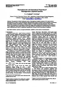
Remark 4.1 Even though it refers to concepts yet to be defined, it is helpful to give the intuitive motivation behind the labelling, If Γ | δ `Θ t : σ is derivable and x ∈ dom(Γ) then δ(x) = 1 implies that the term t is strict in x in the following sense. Given closed terms {sy }y∈dom(Γ) , of appropriate types, then, in any evaluation of a term of the form E[t[sy /y]y∈dom(Γ) ], where E[·] is a ground evaluation context expecting an argument of type σ, it must hold that at least one occurrence of sx is evaluated. If instead δ(x) = 0 then no guarantees are available about the operational behaviour of t with respect to terms substituted for x.

2. (Uniformity) For any domain (B, {rpB }p ), and functions f : A → A, g : B → B and strict h : A ( B, if g ◦ h = h ◦ f then fixB (g) = h(fixA (f )). Remark 3.6 Given Axiom 2, Axiom 4 is again inconsistent with classical logic as it implies the existence of nontrivial sets for which every endofunction has a fixed point. Remark 3.7 It can be shown, see e.g. [23], that fixA is uniquely determined by the property of uniformity. Moreover, by the dinaturality property of loc. cit., fixA does not depend on the algebra structure {rp }p .

The typing rules are given in Figure 1, and are to be read as applying only when the premises and conclusion are all 4

Γ | 0, x : 1 σ `Θ x : σ

Γ | δ, x : 1 σ `Θ t : τ

(var)

Γ | δ `Θ λx : σ. t : σ ( τ

Γ | δ `Θ t : σ Γ | 0 `Θ ! t : ! σ Γ | δ `Θ,α t : σ Γ | δ `Θ Λα. t : ∀α. σ

(bang)

(Lam)

(lam)

Γ | δ `Θ s : ! σ

Γ | δ `Θ s : σ ( τ

Γ | δ ∨ δ 0 `Θ s(t) : τ Γ | δ 0 , x : σ `Θ t : τ

Γ | δ ∨ δ 0 `Θ let !x = s in t : τ Γ | δ `Θ t : ∀α. σ

Γ | δ `Θ t(τ ) : σ[τ /α]

Γ | δ 0 `Θ t : σ

(let)

Γ | δ, x : σ `Θ t : σ

(App)

(app)

Γ | δ `Θ rec x : σ. t : σ

(rec)

Figure 1. Typing Rules s ⇓s λx : σ. s0 λx : σ. t ⇓ λx : σ. t s ⇓ ! s0 !t ⇓ !t

t ⇓s v 0

s0 [v 0 /x] ⇓s v

s(t) ⇓s v

s0 [t/x] ⇓n v

s(t) ⇓n v t ⇓ Λα. t0

t[s0 /x] ⇓ v

let !x = s in t ⇓ v

s ⇓n λx : σ. s0

Λα. t ⇓ Λα. t

t0 [σ/α] ⇓ v

t(σ) ⇓ v

t[rec x : σ. t / x] ⇓ v rec x : σ. t ⇓ v

Figure 2. Evaluation relations well formed. The rules make use of the following notation. We write Θ, α to mean Θ ∪ {α}, where we assume that α ∈ / Θ. Under the assumption that x ∈ / dom(Γ), we write Γ | δ, x : 0 σ for the context consisting of the type assignment Γ, x : σ and the labelling δ[0/x]. Similarly, we write Γ | δ, x : 1 σ for the context consisting of the type assignment Γ, x : σ and the labelling δ[1/x]. The notation Γ | δ, x : σ is used to represent either of the contexts Γ | δ, x : 0 σ and Γ | δ, x : 1 σ. We also make use of the join semilattice operations on labellings of Γ under the pointwise ordering (where the ordering on {0, 1} is 0 ≤ 1). We write: 0 for the least labelling of Γ (the everywhere 0 labelling); and δ ∨ δ 0 for the join of δ and δ 0 .

the intuitionistic/linear divide is stronger than the contraction (within the linear context itself) of relevant logic. We believe that our form of contraction is the natural one for dealing with strictness issues. Given that strictness (as opposed to linearity) is often the important issue in determining an efficient evaluation strategy, it is plausible that languages based on our contraction principle might serve as useful intermediate languages in compilation, e.g. as target languages for strictness analysis.

Remark 4.2 Our language relates to the language Lily of [2] as follows. Given a term Γ; ∆ `Θ t : σ of Lily, where Γ; ∆ is a “dual” intuitionistic/linear context, there exists a (unique) labelling δ of the concatenated context Γ, ∆ such that δ(x) = 1 for all x ∈ dom(∆) and Γ, ∆ | δ `Θ t : σ.2 Thus every term typable in Lily has a type in our language. The converse fails. In fact, our language is equivalent to extending Lily with a contraction principle that contracts Γ, x : σ; y : σ, ∆ `Θ t : σ to Γ; y : σ, ∆ `Θ t[y/x] : σ. Such contraction across

Lemma 4.3 If both Γ | δ `Θ t : σ and Γ | δ 0 `Θ t : σ 0 then δ = δ 0 and σ = σ 0 .

The reason for formulating the typing rules as we have (rather than, e.g., using an explicit contraction rule) is so that the rules are syntax directed. In fact, labellings as well as types are uniquely determined by terms and contexts.

As in [2], we give two operational semantics to our language. In both, values are closed terms of the form: v ::= λx : σ. t | ! t | Λα. t . Figure 2 defines evaluation relations t ⇓s v and t ⇓n v between closed terms t and values v. The strict (or call-byvalue) relation t ⇓s v is inductively defined by the specific ⇓s rule for application together with all rules written using the neutral ⇓ notation. Similarly, the non-strict (or call-byname) relation t ⇓n v is defined by the ⇓n application rule

2 We are ignoring the inessential syntactic difference between the recursively defined thunks of [2] and our explicit recursion operator, as the two are interdefinable, see op. cit.

5

3. if t vsapp t0 : ∀α. σ then, for all closed τ , it holds that t(τ ) vsapp t0 (τ ) : σ[τ /α].

together with the neutral rules. We write t ⇓s (resp. t ⇓n ) to mean that there exists v such that t ⇓s v (resp. t ⇓n v). We write t 's t0 for strict Kleene equality: t ⇓s v iff t0 ⇓s v. Both semantics are easily seen to be deterministic: if t ⇓s v and t ⇓s v 0 then v = v 0 (and similarly for ⇓n ). Also, both are type sound: if t : σ and t ⇓s v then v : σ (and similarly for ⇓n ), where we write t : σ to mean that t is a closed term of closed type σ. As in [2], we define contextual (approximation and) equivalence using termination at types of the form ! σ as observations. In natural extensions of the language with additional type primitives, this turns out to be equivalent to observing termination at ground types only. This choice has many benefits, including: inducing extensionality properties for function and universal types, and the operational correctness of Plotkin’s polymorphic encodings of type constructs. See [2] for a thorough discussion of these issues for the language Lily. For closed σ, a ground σ-context is a term of the form x : σ ` C : ! τ . We usually denote such a context by C[·], and write C[t] for C[t/x], where t : σ.

Strict applicative simulation has an alternative, more elementary, characterization. A ground evaluation context is a ground context generated by the grammar below: E[·] ::= [·] | E[(·)(V )] | E[(·)(τ )] | let !x = (·) in E[x] . Proposition 4.8 If t, t0 : σ then t vsapp t0 iff E[t] ⇓s implies E[t0 ] ⇓s for all ground evaluation σ-contexts E[·]. Theorem 4.9 (Operational extensionality) If t, t0 : σ then t vgnd t0 if and only if t vsapp t0 . Again, we prove this theorem in Section 7.

5. A Relationally Parametric Model In this section, we construct a relationally parametric model of our language. To do this, we give two interpretations of types: as domains, and as relations. For D a domain, a subdomain of D is any subpointed subset D0 ⊆ D that is also a predomain. If D, E are domains then an admissible relation between D and E is a subdomain of the domain D × E. We write R(D, E) for the set of all admissible relations.

Definition 4.4 (Contextual approximation/equivalence) For t, t0 : σ, we write t vgnd t0 to mean that, for all ground σ-contexts it holds that C[t] ⇓s implies C[t0 ] ⇓s . We write t ≡gnd t0 to mean that both t vgnd t0 and t0 vgnd t hold.

Lemma 5.1 If D, E are domains and f : D ( E then

We do not introduce a non-strict variant of contextual approximation, because it follows from the theorem below that this coincides with the strict version above. s

graph(f ) = {(d, e) | f (d) = e} is an admissible relation between D and E.

n

In particular, for any domain D, the diagonal relation ∆D = {(x, x) | x ∈ D} = graph(idD ) is admissible. Given a set of type variables Θ, a Θ-environment is a function γ : Θ → Dom, and a relational Θ-environment is a tuple γR = (γ1Q , γ2 , γR ), where γ1 , γ2 are Θenvironments, and γR ∈ α∈Θ R(γ1 (α), γ2 (α)). For each type σ(Θ) and Θ-environment γ, we define a domain [[σ]]γ and, for each relational Θ-environment γR , we define an admissible relation [[σ]]R γR ∈ R([[σ]]γ1 , [[σ]]γ2 ). The interdependent definitions are given in Figure 3. In them, we write ∆R γ for the relational Θ-environment (γ, γ, α 7→ ∆γ(α) ) determined by a Θ-environment γ. That these definitions are good can be shown using Axiom 2. The relational interpretation of types implies that open types act functorially on the (large) groupoid of strict isomorphisms between domains, cf. [10, 3].

Theorem 4.5 (Strictness) If t : ! σ then t ⇓ iff t ⇓ . We shall prove this theorem in Section 7. Until we have the proof, the reader must keep in mind that vgnd and ≡gnd are defined using the strict evaluation relation. Remark 4.6 Because Lily is included in our language, the strictness theorem for Lily [2, Theorem 2.3] is a consequence of Theorem 4.5 above. Contextual approximation and equivalence can be hard to reason with directly. To address this, we introduce a complementary applicative (bi)simulation relation, which is more amenable to certain forms of argument, and we prove operational extensionality: the coincidence of ground contextual approximation and applicative simulation. Definition 4.7 (Strict applicative simulation) The relation vsapp is the largest relation between closed terms of identical closed type satisfying:

Lemma 5.2 (Groupoid action) If σ(Θ, α) then, for any Θ-environment γ, domains D1 , D2 and isomorphism i : D1 ( D2 , there exists a unique isomorphism gpd(σ, γ, i) : [[σ]]γ[D1 /α] ( [[σ]]γ[D2 /α] such that

1. if t vsapp t0 : σ ( τ then, for all values v : σ, it holds that t(v) vsapp t0 (v) : τ ;

[[σ]]R = graph(gpd(σ, γ, i)). ∆R γ [(D1 ,D2 ,graph(i))/α]

2. if t vsapp t0 : ! σ then t ⇓s ! s implies t0 ⇓s ! s0 where s vsapp s0 : σ; and

Moreover, the mapping i 7→ gpd(σ, γ, i) is functorial. 6

[[α]]γ = γ(α) [[σ ( τ ]]γ = [[σ]]γ ( [[τ ]]γ [[! σ]]γ = L[[σ]]γ Y [[∀α. σ]]γ = {π ∈ [[σ]]γ[D/α] | ∀D1 , D2 ∈ D, ∀R ∈ R(D1 , D2 ), [[σ]]R ∆γ [R/α] (πD1 , πD2 )} D∈D

[[α]]R γR (d1 , d2 ) ⇔ γR (α)(d1 , d2 ) R R [[σ ( τ ]]R γR (f1 , f2 ) ⇔ ∀d1 ∈ [[σ]]γ1 , d2 ∈ [[σ]]γ2 , [[σ]]γR (d1 , d2 ) → [[τ ]]γR (f1 (d1 ), f2 (d2 )) R [[! σ]]R γR (e1 , e2 ) ⇔ (∀d1 ∈ [[σ]]γ1 , e1 = {d1 } → ∃d2 ∈ [[e2 ]]γ2 , [[σ]]γR (d1 , d2 ) ) ∧

(∀d2 ∈ [[σ]]γ2 , e2 = {d2 } → ∃d1 ∈ [[e1 ]]γ1 , [[σ]]R γR (d1 , d2 ) ) R [[∀α. σ]]R γR (π1 , π2 ) ⇔ ∀D1 , D2 ∈ D, ∀R ∈ R(D1 , D2 ), [[σ]]γR [R/α] (πD1 , πD2 ) .

Figure 3. Interpretation of Types [[x]]γ,ρ [[λx : σ. t]]γ,ρ [[s(t)]]γ,ρ [[! t]]γ,ρ [[let !x = s in t]]γ,ρ [[Λα. t]]γ,ρ [[t(τ )]]γ,ρ [[rec x : σ. t]]γ,ρ

= ρ(x) = (d : [[σ]]γ 7→ [[t]]γ,ρ[d/x] ) = [[s]]γ,ρ ([[t]]γ,ρ ) = {[[t]]γ,ρ } = (d : [[σ]]γ 7→ [[t]]γ,ρ )∗ ([[s]]γ,ρ ) = {[[t]]γ[D/α],ρ }D∈D = gpd(σ, γ, i)(([[t]]γ,ρ )D ) where D ∈ D and i : D ( [[τ ]]γ is iso = fix(d : [[σ]]γ 7→ [[t]]γ,ρ[d/x] ) Figure 4. Interpretation of Terms

Corollary 5.3 (Identity extension) For any type σ(Θ) and Θ-environment γ, [[σ]]R ∆R = ∆[[σ]]γ .

3. (Relational parametricity) For any relational Θenvironment γR , any Γ-γ1 -environment ρ1 and Γ-γ2 environment ρ2 , define

γ

Identity extension implies that all elements in the interpretation of polymorphic types ∀α. σ are relationally parametric. Next, we define the interpretation of terms. Given a Θcontext Γ and Q a Θ-environment γ, then a Γ-γ-environment is any ρ ∈ x∈dom(Γ) [[Γ(x)]]γ . A term Γ | δ `Θ t : σ is interpreted as an element [[t]]γ,ρ ∈ [[σ]]γ , relative to any Θ-environment γ and Γ-γ-environment ρ. The definition of [[t]]γ,ρ is given in Figure 4, where terms and subterms are assumed to have the types given in Figure 1.

[[Γ]]γR (ρ1 , ρ2 ) ⇔ ∀x ∈ dom(Γ), [[Γ(x)]]γR (ρ1 (x), ρ2 (x)). Then [[Γ]]γR (ρ1 , ρ2 ) implies [[σ]]γR ([[t]]γ1 ,ρ1 , [[t]]γ2 ,ρ2 ). Remark 5.5 The form of completeness that holds for the small category D (see Remark 3.1) is too weak for interpreting polymorphism in D, see [16]. We side-step the problem by, instead, using the non-small (but properly complete) category Dom for the interpretation. The one difficulty that arises lies in interpreting type specialization. For this, the invariance of the interpretation of universal types under groupoid action, cf. [10, 3], which follows from parametricity, is crucial to showing that the definition of [[t(τ )]]γ,ρ given in Figure 4 is independent of the choice of i and D.

Lemma 5.4 (Interpretation of terms) If Γ | δ `Θ t : σ: 1. (Well-definedness) For any Θ-environment γ and Γ-γenvironment ρ, the value [[t]]γ,ρ ∈ [[σ]]γ is well-defined. 2. (Strictness) If x : τ ∈ Γ and δ(x) = 1 then for any Θ-environment γ and Γ-γ-environment ρ, the function d 7→ [[t]]γ,ρ[d/x] : [[τ ]]γ → [[σ]]γ is strict.

Remark 5.6 Birkedal, Mogelberg and Petersen3 have been 3 Private

7

communication.

d αζ t ⇔ d α t f σζ1 (σ2 s ⇔ f ↓ → (s ⇓s λx : σ1 . s0 and ∀d ∈ [[σ1 ]]γ , ∀t : σ1 [~τ /Θ], d σζ1 t → f (d) σζ2 s0 [t/x]) e !ζσ t ⇔ ∀d ∈ [[σ]]γ , e = {d} → (∃t0 : σ, t ⇓s ! t0 and d σζ t0 ) σ π ∀α. t ⇔ π ↓ → (t ⇓s Λα. t0 and ∀D ∈ D, ∀τ, ∀  ∈ As (D, τ ), πD σζ[(D,τ,)/α] t0 [τ /α]) ζ

Figure 5. Interpretation of Types as Strict Approximation Relations studying a domain-theoretic version of the “parametric completion” process of [17]. It would be interesting to compare the category-theoretic model they obtain with the environment model constructed here.

concretely with PER models. Our language, with its treatment of strictness, is more refined than Amadio’s (e.g., ours supports Plotkin’s encodings of datatypes), and our proof works within the purely axiomatic setting of this paper. The crucial point in formulating a usable notion of approximation relation is the identification of a suitable notion of “definedness” for an arbitrary domain D. For d ∈ D, we write d ↓ to mean that there exists a strict function t : D ( Σ such that t(d). For a domain D and closed type σ, a strict approximation relation between D and σ is a relation  between elements of D and closed terms of type σ satisfying:

Having constructed a relationally parametric model, we could, at this point, go on to prove useful consequences of parametricity. One of the most important consequences is the correctness of Plotkin’s impredicative encodings of the domain-theoretic type constructors (see [2] for details of the encodings, and for a proof of correctness for coproducts). However, for lack of space, and because the techniques needed for such applications of parametricity are known, we omit reworking the expected verifications in our setting. Instead, for the remainder of the paper, we concentrate on showing how our model can be used to prove operational properties of our language. In particular, we obtain denotational proofs of Theorems 4.5 and 4.9.

(sa1) {d | d  t} is a subdomain of D. (sa2) If d ↓ implies d  t then d  t. (sa3) If d  t and t 's t0 then d  t0 . (sa4) If d  t and d ↓ then t ⇓s . We write As (D, σ) for the set of all strict approximation relations between D and σ. Given a set of type variables Θ, a Θ-substitution is a family ~τ = {τα }α∈Θ of closed types. For a type σ(Θ), we write σ[~τ /Θ] for the evident closed type resulting from the substitution. A strict approximation Θ-environment is a triple ζ = (γ, ~τ , {α }α∈Θ ), where γ is a Θ-environment, ~τ is a Θ-substitution and α ∈ As (γ(α), τα ). For any type σ(Θ) and strict approximation Θ-environment ζ = (γ, ~τ , {α }α ), Figure 5 defines a strict approximation relation σζ ∈ As ([[σ]]γ , σ[~τ /Θ])

6. Computational Adequacy In order to use our model to prove operational properties, it is necessary to prove computational adequacy. For x, y in a set X, we write x vΣ y to mean that, for all t : X → Σ, it holds that t(x) implies t(y). The vΣ relation is a preorder (but not necessarily a partial order). Theorem 6.1 (Computational adequacy) The following equivalent properties all hold.

Remark 6.2 It takes quite some work to verify that σζ , is indeed a strict approximation relation. In fact, this is the first place in the paper that property 4 of Axiom 2 is used.

1. If t : ! σ then t ⇓s if and only if ∃d ∈ [[σ]], [[t]] = {d}. 2. If s, t : σ then [[s]] vΣ [[t]] implies s vgnd t. 3. If s, t : σ then [[s]] = [[t]] implies s ≡gnd t.

Remark 6.3 To the reader acquainted with proofs of computational adequacy, the use of substitutions s0 [t/x] for arbitrary terms t rather than just values, in the definition of σζ1 (σ2 , may appear to conflict with the strict operational semantics. However, for our language, the proof of computational adequacy is insensitive to this issue: one could indeed restrict to values, but there is no need to do so.

We prove statement 1. The left-to-right implication is easily shown by proving that t ⇓s v implies [[t]] = [[v]], by induction on the evaluation relation. The converse implication is proved by constructing an “approximation relation” between syntax and semantics. The construction is reminiscent of Girard’s method of proving strong normalization for the polymorphic λ-calculus, see e.g. [4]. A similar approach to computational adequacy for a polymorphic language was previously taken by Amadio [1], who worked

Given a Θ-context Γ and a Θ-substitution ~τ , a Γ-~τ substitution is a family ~t = {tx : Γ(x)[~τ /Θ]}x∈dom(Γ) . 8

d -αζ t ⇔ d -α t f -σζ1 (σ2 s ⇔ ∀d ∈ [[σ1 ]]γ , ∀t : σ1 [~τ /Θ], d -σζ1 t → f (d) -σζ2 s(t) e -!ζσ t ⇔ ∀d ∈ [[σ]]γ , e = {d} → (∃t0 : σ, t ⇓n ! t0 and d -σζ t0 ) σ π -∀α. t ⇔ ∀D ∈ D, ∀τ, ∀ - ∈ An (D, τ ), πD -σζ[(D,τ,-)/α] t(τ ). ζ

Figure 6. Interpretation of Types as Non-strict Approximation Relations Lemma 6.4 Suppose Γ | δ `Θ s : σ. For any strict approximation Θ-environment ζ = (γ, ~τ , {α }α ), for any Γγ-environment ρ and Γ-~τ -substitution ~t, define

For a domain D and closed type σ, a non-strict approximation relation between D and σ is a relation - between elements of D and closed terms of type σ satisfying: (na1) {d | d - t} is a subdomain of D. (na2) If d ↓ implies d - t then d - t. (na3) If d - t and t vnapp t0 then d - t0 .

Γ(x) ρ Γζ ~t ⇔ ∀x ∈ dom(Γ), ρ(x)  ζ tx .

Then ρ Γζ ~t implies [[s]]γ,ρ σζ s[~τ /Θ][~t/Γ].

We write An (D, σ) for the set of all non-strict approximation relations between D and σ. A non-strict approximation Θ-environment is a triple ζ = (γ, ~τ , {-α }α∈Θ ), where γ is a Θ-environment, ~τ is a Θ-substitution and -α ∈ An (γ(α), τα ). For any type σ(Θ) and non-strict approximation Θ-environment ζ = (γ, ~τ , {-α }α ), Figure 6 defines a relation -σζ ∈ An ([[σ]]γ , σ[~τ /Θ]). (Again, it takes quite some work to show that the definition is good.)

As usual, the lemma is proved by induction on s. By the lemma, if s : σ then [[s]] σ s. The right-to-left implication of Theorem 6.1.1 follows.

7. Further Operational Properties The goal of this section is to prove the strictness and operational extensionality theorems claimed in Section 4. For this, we define a second approximation relation between syntax and semantics. If the strictness theorem alone were our goal then it would be possible to simply modify the definitions of Section 6 by systematically replacing strict evaluation with non-strict evaluation.4 However, in order to prove operational extensionality, we need a more substantial alteration. Our proof adapts the technique of [11], where (in essense) operational extensionality for recursively typed languages is addressed, to the more expressive setting of our polymorphic language.

Lemma 7.2 Suppose Γ | δ `Θ s : σ. For any non-strict approximation Θ-environment ζ = (γ, ~τ , {-α }α ), for any Γ-γ-environment ρ and Γ-~τ -substitution ~t, define Γ(x) ρ -Γζ ~t ⇔ ∀x ∈ dom(Γ), ρ(x) - ζ tx .

Then ρ -Γζ ~t implies [[s]]γ,ρ -σζ s[~τ /Θ][~t/Γ]. Again, the proof is by induction on s. The lemma establishes, in particular, that if s : σ then [[s]] -σ s. Corollary 7.3 (Non-strict computational adequacy) If t : ! σ then t ⇓n if and only if ∃d ∈ [[σ]], [[t]] = {d}.

Definition 7.1 (Non-strict applicative simulation) The relation vnapp is the largest relation between closed terms of identical closed type satisfying:

Theorem 4.5 (the strictness theorem) is an immediate consequence of the above corollary and Theorem 6.1.1.

1. if t vnapp t0 : σ ( τ then, for all terms s : σ, it holds that t(s) vnapp t0 (s) : τ ;

Lemma 7.4 If t, t0 : σ then [[t]] -σ t0 iff t vnapp t0 . Proof (sketch). Using Lemma 7.2, one shows that the relation [[t]] -σ t0 satisfies implications 1–3 of Definition 7.1. So [[t]] -σ t0 implies t vnapp t0 . Conversely, if t vnapp t0 then, by Lemma 7.2, [[t]] -σ t. So, by (na3), [[t]] -σ t0 . 2

2. if t vnapp t0 : ! σ then t ⇓n ! s implies t0 ⇓n ! s0 where s vnapp s0 : σ; and 3. if t vnapp t0 : ∀α. σ then, for all closed τ , it holds that t(τ ) vnapp t0 (τ ) : σ[τ /α].

Proposition 7.5 If t, t0 : σ then t vgnd t0 iff t vnapp t0 iff t vsapp t0 .

4 To prove adequacy for the non-strict semantics, the quantification over arbitrary terms t in the definition of σζ1 (σ2 is crucial; cf. Remark 6.3.

9

Proof (sketch). Using Theorem 4.5, it is not hard to show that the relation t vgnd t0 satisfies implications 1–3 of Definition 4.7. So t vgnd t0 implies t vsapp t0 . Using the characterization of Proposition 4.8, and Theorem 4.5, one can show that t vsapp t0 satisfies 1–3 of Definition 7.1, so t vsapp t0 implies t vnapp t0 . It remains to show that t vnapp t0 implies t vgnd t0 . Suppose t vnapp t0 . By Theorem 4.5, it suffices to show that x : σ ` C[x] : ! τ implies C[t] vnapp C[t0 ]. By Lemma 7.4, [[t]] -σ t0 . If x : σ ` C[x] : ! τ then [[C[t]]] = [[C]][[[t]]/x] -σ C[t0 ], by Lemma 7.2. So, by Lemma 7.4, indeed C[t] vnapp C[t]. 2

[3] P. J. Freyd, E. P. Robinson, and G. Rosolini. Functorial Parametricity. In Proc. 7th Symposium on Logic in Comp. Sci., pages 444–452, Santa Cruz, 1992. [4] J.-Y. Girard, P. Taylor, and Y. Lafont. Proofs and Types. Cambridge University Press, 1989. [5] J. M. E. Hyland. A small complete category. Annals of Pure and Applied Logic, 40:135 – 165, 1988. [6] J. M. E. Hyland. First steps in synthetic domain theory. In Category Theory, Proc. Como 1990, pages 131–156. Springer LNM 1488, 1991. [7] J. M. E. Hyland, E. P. Robinson, and G. Rosolini. The discrete objects in the effective topos. Proc. Lond. Math. Soc., 3(60), 1990. [8] J. R. Longley and A. K. Simpson. A uniform account of domain theory in realizability models. Math. Struct. in Comp. Sci., 7:469–505, 1997. [9] W. K.-S. Phoa. Effective domains and intrinsic structure. In Proc. 5th Annual Symposium on Logic in Comp. Sci., pages 366–377, 1990. [10] W. K.-S. Phoa. Two reults on set-theoretic polymorphism. In Category Theory in Comp. Sci., pages 219–235. Springer LNCS 530, 1991. [11] A. M. Pitts. A note on logical relations between semantics and syntax. Logic Journal of the Interest Group in Pure and Applied Logics, 5(4):589–601, 1997. [12] G. D. Plotkin. Type theory and recursion. Invited talk at 8th Symposium on Logic in Comp. Sci., 1993. [13] G. D. Plotkin and A. J. Power. Computational effects and operations: an overview. Elect. Notes in Theor. Comp. Sci., to appear, 2004. [14] B. Reus and T. Streicher. General synthetic domain theory — a logical approach. Math. Struct. in Comp. Sci., 9:177– 223, 1999. [15] J. C. Reynolds. Types, abstraction and parametric polymorphism. In Information Processing ’83, pages 513–523. North Holland, 1983. [16] E. P. Robinson. How complete is PER? In Proc. 4th Symposium on Logic in Comp. Sci., pages 106–111, 1989. [17] E. P. Robinson and G. Rosolini. Reflexive graphs and parametric polymorphism. In Proc. 9th Symposium on Logic in Comp. Sci., pages 364–371, 1994. [18] G. Rosolini. Continuity and Effectivity in Topoi. PhD thesis, University of Oxford, 1986. ˇ cedrov. Intuitionistic set theory. In Harvey Friedman’s [19] A. S˘ Research on The Foundations of Mathematics, pages 257– 284. Elsevier Science Publishers, 1985. [20] D. S. Scott. Relating theories of the λ-calculus. In J. Seldin and J. Hindley, editors, To H.B. Curry: Essays on Combinatory Logic, Lambda Calculus and Formalism, pages 403– 450. Academic Press, 1980. [21] A. K. Simpson. Computational adequacy in an elementary topos. In Comp. Sci. Logic, Proc. CSL ’98, pages 323–342. Springer LNCS 1584, 1999. [22] A. K. Simpson. Computational adequacy for recursive types in models of intuitionistic set theory. In Proc. 17th Symposium on Logic in Comp. Sci., pages 282–298, 2002. [23] A. K. Simpson and G. D. Plotkin. Complete axioms for categorical fixed-point operators. In Proc. 15th Symposium on Logic in Comp. Sci., pages 30–41, 2000.

Theorem 4.9 is an immediate consequence.

8. Justification In this section, we briefly justify the correctness of our methods for establishing operational properties. All our axioms and arguments can be interpreted within any realizability topos E satisfying the strong completeness axiom of [8], by taking predomains to be the well-complete objects. In op. cit. it is explicitly shown that Axioms 1, 2 and 4 of this paper are consequences of strong completeness. Moreover, the validity of Axiom 3 follows from the results of [7]. Thus all results of this paper are true when interpreted within E. It remains to argue that all results with operational content are true in reality. For this, we observe the following. The evaluation relations t ⇓s , t ⇓s v, t ⇓n and t ⇓n v are all Σ01 . Consequently, the statements t vgnd t0 and t ≡gnd t0 are Π02 . Similarly, t vsapp t0 is Π02 , via the characterization of Proposition 4.8. The statement of the strictness theorem (Theorem 4.5) is a bi-implication between Σ01 formulas, and thus also Π02 . The statement of operational extensionality (Theorem 4.9) is a universally quantified bi-implication between Π02 formulas. It is easily shown that a Π02 sentence holds internally in E if and only if it is true in reality (for the right-to-left implication, an unbounded search provides the realizer). It follows that implications between Π02 statements that are valid in E are also true in reality. Therefore, any operational conclusion of one of the forms discussed above, obtained as a result of the methods of this paper, is indeed true.

References [1] R. Amadio. On the adequacy of PER models. In Mathematical Foundations of Comp. Sci. 1993, pages 222–231. Springer LNCS 711, 1993. [2] G. M. Bierman, A. M. Pitts, and C. V. Russo. Operational properties of Lily, a polymorphic linear lambda calculus with recursion. Elect. Notes in Theor. Comp. Sci., 41, 2000.

10