Using Term Informativeness for Named Entity Detection Jason D. M. Rennie
Tommi Jaakkola
Computer Science and Artificial Intelligence Lab Massachusetts Institute of Technology Cambridge, MA 02139
Computer Science and Artificial Intelligence Lab Massachusetts Institute of Technology Cambridge, MA 02139
[email protected]
[email protected]
ABSTRACT Informal communication (e-mail, bulletin boards) poses a difficult learning environment because traditional grammatical and lexical information are noisy. Other information is necessary for tasks such as named entity detection. How topic-centric, or informative, a word is can be valuable information. It is well known that informative words are best modeled by “heavy-tailed” distributions, such as mixture models. However, informativeness scores do not take full advantage of this fact. We introduce a new informativeness score that directly utilizes mixture model likelihood to identify informative words. We use the task of extracting restaurant names from bulletin board posts as a way to determine effectiveness. We find that our “mixture score” is weakly effective alone and highly effective when combined with Inverse Document Frequency. We compare against other informativeness criteria and find that only Residual IDF is competitive against our combined IDF/Mixture score.
Categories and Subject Descriptors I.2.7 [Artificial Intelligence]: Natural Language Processing; I.2.6 [Artificial Intelligence]: Learning
General Terms Algorithms
Keywords Named Entity Extraction, Inverse Document Frequency, Mixture Models, Term Frequency Distribution
1.
INTRODUCTION
We are interested in the problem of extracting information from informal, written communication. At the time of this writing, Google.com catalogs eight billion web pages. There are easily that number of e-mail, newsgroup and bulletinboard posts each day. The web is filled with information,
Permission to make digital or hard copies of all or part of this work for personal or classroom use is granted without fee provided that copies are not made or distributed for profit or commercial advantage and that copies bear this notice and the full citation on the first page. To copy otherwise, to republish, to post on servers or to redistribute to lists, requires prior specific permission and/or a fee. SIGIR’05, August 15–19, 2005, Salvador, Brazil. Copyright 2005 ACM 1-59593-034-5/05/0008 ...$5.00.
but even more information is available in the informal communications people send and receive on a day-to-day basis. We call this communication informal because structure is not explicit and the writing is not fully grammatical. Web pages are highly structured. They use links, headers and tags to mark-up the text and identify important pieces of information. Newspaper text is harder to deal with. Gone is the computer-readable structure. But, newspaper articles have proper grammar with correct punctuation and capitalization; part-of-speech taggers show high accuracy on newspaper text. In informal communication, even these basic cues are noisy—grammar rules are bent, capitalization may be ignored or used haphazardly and punctuation use is creative. There is good reason why little work has been done on this topic: the problem is challenging and data can be difficult to attain due to privacy issues. Yet, the volume of informal communication that exists makes us believe that trying to chip away at the information extraction problem is a useful endeavor. Restaurants are one subject where informal communication is highly valuable. Much information about restaurants can be found on the web and in newspaper articles. Zagat’s publishes restaurant guides. Restaurants are also discussed on mailing lists and bulletin boards. When a new restaurant opens, it often takes weeks, or months before reviews are published on the web or in the newspaper (Zagat’s guides take even longer). However, restaurant bulletin boards contain information about new restaurants almost immediately after they open (sometimes even before they open). They are also “up” on major changes: a temporary closure, new management, better service or a drop in food quality. This information is difficult to find elsewhere. This timely information can be difficult to extract. Systems that extract named entities from newspaper articles rely heavily on capitalization, punctuation and correct partof-speech information. In informal communication, much of this information is noisy—other features need to be incorporated. An important sub-task of extracting information from restaurant bulletin boards is identifying restaurant names. It has been found that named entities, like restaurant names, are highly relevant to the topic of a document [6]. If we had a good measure of how topic-oriented, or “informative,” each word was, we would be better able to identify named entities. It is well known that informative words have “peaked” or “heavy-tailed” frequency distributions [5]. Many informativeness scores have been introduced, including Inverse Document Frequency (IDF) [11], Residual IDF [4], xI [2], the z-measure [8] and Gain [12]. Only xI
makes direct use of the fit of a word’s frequency statistics to a peaked/heavy-tailed distribution. However, xI does a poor job of finding informative words. We introduce a new informativeness score that is based on the fit of a word’s frequency statistics to a mixture of 2 Unigram distributions. We find that it is effective at identifying topic-centric words. We also find that it combines well with IDF. Our combined IDF/Mixture score is highly effective at identifying informative words. In our restaurant extraction task, only one other informativeness score, Residual IDF, is competitive. Using Residual IDF or our combined IDF/Mixture score, our ability to identify restaurant names is significantly better than using capitalization, punctuation and part-of-speech information alone. In more formal or structured settings, informativeness may be of marginal use, but here we find it to be of great value.
2.
INFORMATIVENESS MEASURES
Inverse document frequency (IDF) is an informativeness score that was originally introduced by Jones [11]. It embodies the principle that the more rare a word is, the greater the chance it is relevant to those documents in which it appears. Specifically, the IDF score for a word, w, is IDF = − log
(docs with w) . (total # docs)
(1)
The IDF score has long been used to weight words for information retrieval. It has also been used with success in text classification [10, 13]. Recently, Papineni [12] showed that the IDF score can be derived as the optimal classification weight for a special self-classification problem using an exponential model and a generalized form of likelihood. In short, IDF has seen much success and has theoretical justification. However, it is a weak identifier of informative words. Since the introduction of IDF, many other informativeness scores have been introduced. Bookstein and Swanson [2] introduce the xI measure for a word w, xI (w) = fw − dw ,
(2)
where fw is the frequency of word w and dw is the document frequency of word w (number of documents in which w occurs). Informative words tend to exhibit “peaked” distributions with most occurrences coming in a handful of documents. This score makes sense at the intuitive level since, for two words with the same frequency, the one that is more concentrated will have the higher score. However, this score has a bias toward frequent words, which tend to be less informative. Harter [8] noted that frequency statistics of informative or “specialty” words tend to fit poorly to a Poisson distribution. He suggested that informative words may be identified by observing their fit to a mixture of 2 Poissons (“2Poisson”) model; he introduced the z-measure as a criterion for identifying informative words. The z-measure, introduced earlier by [3], is a general measure between two distributions. It computes the difference between means divided by square-root of the summed variances: µ1 − µ2 z= p 2 (3) σ1 + σ22 Harter found that this measure could be used to identify informative words for keyword indexing.
Twenty years later, Church and Gale [4] noted that nearly all words have IDF scores that are larger than what one would expect according to an independence-based model (such as the Poisson). They note that interesting or informative should tend to have the largest deviations from what would be expected. They introduced the Residual IDF score, which is the difference between the observed IDF and the IDF that would be expected: [. Residual IDF = IDF − IDF
(4)
The intuition for this measure is similar to that of Bookstein and Swanson’s xI -measure. Words that are clustered in few documents will tend to have higher Residual IDF scores. However, whereas xI has a bias toward high-frequency words, Residual IDF has the potential to be largest for mediumfrequency words. As such, it serves as a better informativeness score. In our experiments, we find that Residual IDF is the most effective individual informativeness score. Recently, Papineni [12] showed that IDF is the “optimal weight of a word with respect to minimization of a KullbackLieber distance.” He notes that the weight (IDF) is different from the importance or “gain” of a feature. He suggests that the gain in likelihood attained by introducing a feature can be used to identify “important” or informative words. He derives the gain for a word w as „ « dw dw dw Gain(w) = − 1 − log , (5) D D D where dw is the document frequency of word w and D is the total number of documents. Extremely rare and extremely common words have low gain. Medium-frequency words have higher gain. A weakness of this measure is that it relies solely on document frequency—it does not take account for “peaked-ness” of a word’s frequency distribution. These informativeness measures represent a variety of approaches to identifying informative words. Only Harter’s z-measure directly makes use of how a word’s frequency statistics fit a heavy-tailed mixture distribution. Yet, our study indicates that the z-measure is a poor identifier of informative words. In the next section, we introduce a new measure based on a word’s fit to a mixture distribution.
3. MIXTURE MODELS It is a given that topic-centric words are somewhat rare. But we think that they also exhibit two modes of operation: (1) a high frequency mode, when the document is relevant to the word, and (2) a low (or zero) frequency mode, when the document is irrelevant. A mixture is well-suited to model this behavior. We think that we can identify informative words by looking at the difference in log-likelihood between a mixture model and a simple unigram model. We propose that informative words can be effectively modeled with mixtures. For each word, we treat each document as a sequence of coin flips, heads (H) representing an occurrence and tails (T) representing a non-occurrence. Consider the following four short “documents”: {{HHH}, {T T T }, {HHH}, {T T T }} The simplest model for sequential binary data (coin flips) is the unigram. For binary data, the unigram uses a single
Token sichuan fish was speed tacos indian sour villa tokyo greek
parameter which represents the chance of heads on each flip: Y h θ i (1 − θ)(ni −hi ) (6) puni (~n, ~h|θ) = i
We use hi for the number of heads and ni for the number of flips per document. The unigram is a poor model for the above data. The maximum likelihood unigram parameter is θ¯ = 0.5 and the data likelihood is 2−12 . The unigram has no capability to model the switching nature of the data. A mixture is a composite model. It randomly selects between a number of component models. The likelihood for a mixture of two unigrams is: Y“ h pmix (~n, ~h|λ, φ1 , φ2 ) = λφ1 i (1 − φ1 )(ni −hi ) + i
(1 − λ)φh2 i (1 − φ2 )(ni −hi )
”
¯ φ¯1 , φ¯2 ) pmix (~h, ~n; λ, . ¯ puni (~h, ~n; θ)
(8)
We use a ratio because we are interested in knowing the comparative improvement of the mixture model over the simple unigram. And, the log-odds ratio grounds the score at zero. The mixture is strictly more expressive than the simple unigram, so we can guarantee that the score will be non-negative.
4.
EXPECTATION-MAXIMIZATION
We use Expectation-Maximization to maximize the likelihood of the mixture model. We avoid a full discussion of EM because it is not essential to the understanding of our contributions. See Dempster et al. for more information [7]. EM uses a bound to iteratively update model parameters to increase likelihood. Since likelihood as a function of mixture parameters is not convex, the maximum EM finds may only be local. To increase our chances of finding a global maximum, we use two starting points: (1) one slightly offset from the unigram model, and (2) one “split” model where the first unigram component is set to zero and the second component and the mixing parameter (λ) are set to otherwise maximize the likelihood of the data. We found that this worked well to find global maxima—extensive random sampling never found a higher likelihood parameter setting.
5.
Rest. 31/52 7/73 0/483 16/19 4/19 3/30 0/31 10/11 7/11 0/20
Token sichuan ribs villa tokyo penang kuay br khao bombay strike
Score 2.67 2.52 2.36 2.36 2.17 1.92 1.92 1.92 1.92 1.77
Rest. 31/52 0/13 10/11 7/11 7/9 0/7 6/7 4/7 6/7 0/6
Table 1: Top Mixture Score (left) and Residual IDF (right) Tokens. Bold-face words occurred at least once as part of a restaurant name.
(7)
¯ = 0.5, φ¯1 = Here, the maximum likelihood parameters are λ 1, φ¯2 = 0 and the data likelihood is 2−4 . In effect, the mixture model makes 4 equi-probable decisions whereas the unigram makes 12 decisions. The two extra parameters of the mixture allow for a much better modeling of the data. When data exhibits two distinct modes of behavior, such as with our coin example, the mixture will yield a much higher data likelihood than the simple unigram. Now we are ready to introduce our new informativeness score. For each word, we find maximum-likelihood parameters for both the unigram and mixture models. Our “Mixture score” is then the log-odds of the two likelihoods: smix = log
Score 99.62 50.59 48.79 44.69 43.77 41.38 40.93 40.36 39.27 38.15
FINDING RESTAURANTS
We think that the Mixture score can serve as an effective term informativeness score. To evaluate the correctness of our belief, we use the task of identifying restaurant names in posts to a restaurant discussion bulletin board. We treat
each thread as a document and calculate various informativeness scores using word-thread statistics. Restaurants are often the topic of discussion and tend to be highly informative words. The task of identifying them serves as a good test ground for any measure that claims to rate informativeness. We collected posts from the board and hand-labeled them. The next section details our findings.
5.1 The Restaurant Data We used as a test-bed posts from a popular restaurant bulletin board. The maintainers of the site moderate the board and lay out a set of ground rules for posting. The people who post are not professional restaurant reviewers. They simply enjoy eating and discussing what they have eaten. Information about restaurants can be found in the discussions that ensue. Major metropolitan areas each have their own bulletin board; other boards are grouped by region. We collected and labeled six sets of threads of approximately 100 posts each from a single board (615 posts total). We used Adwait Ratnaparkhi’s MXPOST and MXTERMINATOR1 software to determine sentence boundaries, tokenize the text and determine part-of-speech. We then handlabeled each token as being part of a restaurant name or not. Labeling of the 56,018 tokens took one person about five hours of time. 1,968 tokens were labeled as (part of) a restaurant name. The number of restaurant tokens per set ranged from 283 to 436. We found 5,956 unique tokens. Of those, 325 were used at least once as part of a restaurant name. We used a separate set of data for developing and debugging our experiment code.
6. INFORMATIVENESS FILTERING Here we explore how the various measures serve as informativeness filters. First, we consider the density of restaurant tokens in the top-ranked words. Both Gain and IDF serve as poor informativeness filters, at least with respect to restaurant names—only occasional restaurant tokens are found in words ranked highest by Gain and IDF. The xI measure ranks some restaurant tokens highly—five of the top 10 words occur at least once as part of a restaurant. However, these tokens only appear in restaurant names very rarely. None of the top 30 xI words occur as part of restaurant names at least 50% of the time. The z-measure serves as a reasonably good informativeness filter—three of the top 1
http://www.cis.upenn.edu/∼adwait/statnlp.html
Rank 1 4 8 9 21 22 23 26 29 30
Token sichuan speed villa tokyo zoe penang pearl dhaba gourmet atasca
Rest. 31/52 16/19 10/11 7/11 10/11 7/9 11/13 8/13 23/27 9/10
Rank 1 3 4 5 7 8 9 12 14 16
Token sichuan villa tokyo penang br khao bombay aroma baja mahal
Rest. 31/52 10/11 7/11 7/9 6/7 4/7 6/7 5/6 3/6 5/6
Table 2: Top Mixture Score (left) and Residual IDF (right) Restaurant Tokens (50%+ restaurant usage) 10 words occur as restaurant tokens and nine of the top 30 words occur in restaurant names at least 50% of the time. Both the mixture score and Residual IDF have high densities of restaurant tokens in their top ranks. Table 1 shows the top 10 words ranked by the Mixture score and Residual IDF. For both measures, seven of the top 10 words are used at least once as part of a restaurant name. Table 2 shows, for each measure, the top 10 words used a majority of the time in restaurant names. Most of the top-ranked Residual IDF words occur a majority of the time in restaurant names. Fewer top Mixture score words are majority used in restaurant names, but those that are occur more often than the top Residual IDF words. Top-ranked words give only a partial view of the effectiveness of an informativeness filter. Next, we look at average and median scores and ranks across our entire corpus. Score Mixture z xI RIDF Gain Baseline IDF
Avg. Rank 505 526 563 858 2461 2978 4562
Med. Rank 202 300 326 636 1527 2978 5014
Table 3: Average and Median Restaurant Token Ranks (lower is better) So far, we have considered the upper-tail of informativeness scores; we have done our counting over unique words, thus overweighting rare ones. Here, we compile statistics across the full set of data and count each restaurant token occurrence separately. For each informativeness score, we compute the score for each unique word and rank the words according to score. Then, for each of the 1,968 tokens labeled as (part of) a restaurant name, we determine the token’s rank. We compute both the average and median ranks of the restaurant tokens. Table 3 gives the average and median ranks of restaurant words for the various informativeness scores. The Mixture score gives the best average and median rank. The z-measure and xI -measure give slightly worse rankings. Residual IDF and Gain are better than the baseline2 , while IDF yields worse rankings than the 2
Baseline average and median rank are what would be expected from a score that assigns values randomly. Note that there are 5,956 unique words; 2,978 is half that number.
baseline. The average and median rank give us a good feel for how well a score works as a filter, but not necessarily as a feature in a natural language system. Next, we discuss an evaluation that may better reflect performance on a real task. Score RIDF IDF Mixture z Gain Baseline xI
Avg. Score 3.21 1.92 2.49 1.10 1.00 1.00 0.33
Med. Score 2.72 3.90 2.89 1.09 1.22 1.00 0.00
Table 4: Average and Median Relative Scores of Restaurant Tokens Now we consider the average and median score of restaurant tokens. For each of the 1,968 tokens labeled as (part of) a restaurant name, we compute the informativeness score. We then take an average or median of those scores. We divide by the average or median score across all 56,018 tokens to attain a “relative” score. We do this so that absolute magnitude of the informativeness score is irrelevant; i.e. multiplication by a constant has no effect. Table 4 shows average and median relative scores for restaurant tokens. Of note is the fact that informativeness scores that produce good average/median ranks do not necessarily produce good average/median scores (e.g. z and xI ). Residual IDF gives the best average relative score; IDF gives the best median relative score. The Mixture score gives the second-best average relative score and second-best median relative score. At this point, it seems sufficiently clear that the z-measure, the xI measure and Gain have relatively little to offer in terms of identifying informative words, at least when compared to Residual IDF, IDF and the Mixture score. We focus on RIDF, IDF and the Mixture score for the remainder of this paper.
6.1 Are Mixture and IDF Independent? To this point, both Residual IDF and the Mixture Score appear to be excellent informativeness scores. Both have a high density of restaurant tokens in their highest ranks; for both measures, average/median ranks/scores are much better than baseline. IDF, however, ranks restaurant words poorly, but yields the best median relative score. Since IDF seems so different from the other two scores, we postulate that it might work well in combination. We look at how well correlated the scores are. If two scores are highly correlated, there is little use in combining them—their combination will be similar to either score individually. However, if two scores are uncorrelated, then they are measuring different sorts of information and may produce a score in combination that is better at identifying informative words than either score individually. First, we consider a very simple test on our restaurant data set: how much overlap is there in highly-rated restaurant words? For each of the scores, we choose a threshold that splits the restaurant words (approximately) in half. We then count the number of restaurant words that score above both thresholds. For scores that are independent of each other, we would expect the joint count to be about half of the individual count. Table 5 gives the individual and
60
50
2.5
50
40 30 20
2 1.5 1 0.5
10 0 0
Mixture Score
3
Residual IDF
Mixture Score
60
1
2
3
4
5
0 0
40 30 20 10
1
2
IDF
3
4
0
5
0
0.5
IDF
1 1.5 Residual IDF
2
2.5
Figure 1: Scatter plots comparing pairs of the IDF, Residual IDF and Mixture scores. Only words that appear at least once within a restaurant name are plotted. RIDF/Mixture shows a high degree of correlation. IDF/RIDF shows some correlation. IDF/Mixture shows relatively little correlation. joint statistics. The Mixture/RIDF and IDF/RIDF combinations both show a substantial degree of dependence. This is not the case for Mixture/IDF. If the Mixture and IDF scores were independent, we would expect a joint count of 176 ∗ 170/325 = 92, almost exactly the joint count that we do observe, 93. This gives us reason to believe that the Mixture and IDF scores may be uncorrelated and may work well in combination. Condition Mixture > 4.0 IDF > 4.0 RIDF > 0.5 Mix > 4.0 and IDF > 4.0 Mix > 4.0 and RIDF > 0.5 IDF > 4.0 and RIDF > 0.5
Restaurant 176/325 170/325 174/325 93/325 140/325 123/325
Table 5: Number of restaurant tokens above score thresholds. Our test provides evidence that the IDF and Mixture scores are independent, but it does not exclude the possibility that there are pockets of high correlation. Next, we consider more traditional measures. Figure 1 shows scatter plots of the pairs of scores. Residual IDF (RIDF) and Mixture show a high degree of correlation—knowledge of RIDF is very useful for attempting to predict Mixture score and vice versa. IDF and RIDF show correlation, at least partially reflecting the fact that IDF bounds RIDF. IDF and Mixture show little relation—there is no clear trend in the Mixture score as a function of IDF. These observations are reflected in correlation coefficients calculated on the data, shown in Table 6. IDF and Mixture are practically uncorrelated, while the other score pairs show substantial correlation. Score Names IDF/Mixture IDF/RIDF RIDF/Mixture
Correlation Coefficient -0.0139 0.4113 0.7380
Table 6: Correlation coefficients for pairs of the IDF, Residual IDF and Mixture scores on restaurant words. IDF and Mixture are effectively uncorrelated in the way they score restaurant words. That the IDF and the Mixture scores would work well
Token sichuan villa tokyo ribs speed penang tacos taco zoe festival
Score 376.97 197.08 191.72 181.57 156.25 156.23 153.05 138.38 134.23 127.39
Restaurant 31/52 10/11 7/11 0/13 16/19 7/9 4/19 1/15 10/11 0/14
Table 7: Top IDF*Mixture Score Tokens Rank 1 2 3 5 6 9 12 16 19 21 23
Token sichuan villa tokyo speed penang zoe denise pearl khao atasca bombay
Restaurant 31/52 10/11 7/11 16/19 7/9 10/11 5/8 11/13 4/7 9/10 6/7
Table 8: Top IDF*Mixture Score Restaurant Tokens (50%+ restaurant usage) together makes sense intuitively. They capture very different aspects of the way in which we would expect an informative word to behave. IDF captures rareness; the Mixture score captures a multi-modal or topic-centric nature. These are both aspects that partially identify informative words. Next we investigate whether a combination score is effective for identifying informative words.
6.2 Combining Mixture and IDF We use the relaxation of the conjunction, a simple product, to combine IDF and Mixture. We denote this by “IDF*Mixture.” Table 7 shows the top 10 tokens according to the IDF*Mixture score. Eight of the top 10 are used as restaurant names. Worth noting is that the other two words (“ribs” and “festival”) were topics of discussions on the restaurant bulletin board. Table 8 gives the ranks of
the top 10 tokens that were used regularly in restaurant names. Compared to the Mixture score, restaurant tokens more densely populate the upper ranks. Ten of the top 23 tokens are regularly used as restaurant names. The trend continues. 100 of the top 849 IDF*Mixture tokens are regularly used in restaurant names, while 100 of the top 945 Mixture tokens are regularly used in restaurant names. However, Mixture catches up and and surpasses IDF*Mixture (in terms of restaurant density) as we continue down the list. This explains why Mixture has better average and median ranks (next paragraph). Score Mixture IDF*Mixture RIDF IDF
Avg. Rank 507 682 858 4562
Med. Rank 202 500 636 5014
Table 9: Average and Median Restaurant Token Ranks
true label
classification +1 −1 +1 tp fn −1 fp tn
Table 11: The contingency table for the binary classification problem. ‘tp’, ‘fn’, ‘fp’, and ‘tn’ are the numbers of true positives, false positives, false negatives and true negatives, respectively. particular threshold, we report the maximum F1 score attained over all threshold values. We call this “F1 breakeven” in reference to a similarity it shares with precision-recall breakeven [10]; the breakeven F1 tends to occur when precision and recall are nearly equal. However, unlike precisionrecall breakeven, F1 breakeven is well-defined.
7.2 Significance
Given two classifiers evaluated on the same test sets, we can determine whether one is better than the other using paired differences. We use the Wilcoxon signed rank test [16]; it imposes a minimal assumption—that the difference Score Avg. Score Med. Score distribution is symmetric about zero. The Wilcoxon test IDF*Mixture 7.20 17.15 uses ranks of differences to yield finer-grained distinctions 2 RIDF 7.54 7.40 than a simple sign test. 2 4.61 8.35 Mixture We use the one-sided upper-tail test, which compares the 2 IDF 2.31 15.19 zero-mean null hypothesis, H0 : θ = 0, against the hypothesis that the mean is greater than zero, H1 : θ > 0. We Table 10: Average and Median Relative Scores of compute a statistic based on difference ranks. Let zi be the Restaurant Tokens. Note that a superscript indiith difference. Let ri be the rank of |zi |. Let ψi be a an cates that the score is raised to the given power. indicator for zi : 1, if zi ≥ 0, Here we give rank and relative score averages for IDF*Mixture. (10) ψi = 0, if zi < 0. Table 9 gives the average and median ranks like before. Mixture still leads, but IDF*Mixture is not far behind. TaThe Wilcoxon signed rank statistic is: ble 10 gives the average and median relative scores. The n relative score is affected by exponentiation, so we compare X zi ψi . (11) T+ = against squared versions of IDF, Mixture and Residual IDF. i=1 IDF*Mixture achieves the best median and is a close second for average relative score. IDF*Mixture appears to be Upper-tail probabilities for the null hypothesis are calcua better informativeness score than either IDF or the Mixlated for each possible value3 . We reject H0 (and accept ture score and very competitive against Residual IDF. In H1 ) if the probability mass is sufficiently small. We use the next section, we describe the set-up for a “real” test: a α = 0.05 as the threshold below which we declare a result named entity (restaurant name) extraction task. to be significant. Table 12 gives the upper-tail probabilities
7.
for a subset of the possible values of T + . Values of 19 and higher are significant at the α = 0.05 level.
NAMED ENTITY DETECTION
So far, we have focused on filtering. In this section, we consider on the task of detecting restaurant names. We use the informativeness scores as features in our classifier and report on how accurately restaurants are labeled on test data.
x 17 18 19 20 21
7.1 Performance Measures The F-measure [15], is commonly used to measure performance in problems where negative examples outnumber positive examples. We use the F1-measure (“F1”), which tp tp , and recall, r = tp+fn : equally weights precision, p = tp+fp F1(p, r) =
2pr . p+r
(9)
F1 varies as we move our classification threshold along the real number line. To eliminate any effects of selecting a
P0 (T + ≥ x) .109 .078 .047 .031 .016
Table 12: Upper-tail probabilities for the null hypothesis.
7.3 Experimental Set-Up We used 6-fold cross-validation for evaluation: for each of the six sets, we used the other five sets as training data for 3
We use values from Table A.4 of Hollander and Wolfe [9].
Baseline IDF Mixture RIDF IDF*RIDF IDF*Mixture
F1 brkevn 55.04% 55.95% 55.95% 57.43% 58.50% 59.30%
Table 13: Named Entity Extraction Performance
IDF Mixture RIDF IDF*RIDF IDF*Mixture
Base. 20 18 20 20 21
IDF 15 19 18 21
Mix 19 18 21
RIDF 16 21
IDF*RIDF 15
Table 14: T + Statistic for F1 Breakeven. Each entry that is 19 or higher means that the score to the left is significantly better than the score above. For example, IDF*Mixture is significantly better than RIDF. our classifier4 . No data from the “test” set was ever used to select parameters for the corresponding classifier. However, since the test set for one fold is used in the training set for another, we note that our significance calculations may be overconfident. For classification, we used a regularized least squares classifier (RLSC) [14] and used a base set of features like those used in [1]. Current, next and previous parts-of-speech (POS) were used, along with current-next POS pairs and previousnext POS pairs. We included features on the current, previous and next tokens indicating various types of location, capitalization, punctuation and character classes (firstWord, lastWord, initCap, allCaps, capPeriod, lowerCase, noAlpha and alphaNumeric). Unlike HMMs, CRFs or MMM networks, RLSC labels tokens independently (like an SVM does). We believe that using a better classifier would improve overall classification scores, but would not change relative performance ranking.
7.4 Experimental Results Table 13 gives the averaged performance measures for six different experimental settings: • Baseline: base features only • IDF: base features, IDF score • Mixture: base features, Mixture score • RIDF: base features, Residual IDF • IDF*RIDF: base features, IDF, RIDF, IDF2 , RIDF2 , IDF*RIDF • IDF*Mixture: base features, IDF, Mixture, IDF2 , Mixture2 , IDF*Mixture 4
To select a regularization parameter, we trained on four of the five “training” sets, evaluated on the fifth and selected the parameter that gave the best F1 breakeven.
Table 14 gives the Wilcoxon signed rank statistic for pairs of experimental settings. IDF and the Mixture score both yield small improvements over baseline. The improvement for IDF is significant. Residual IDF serves as the best individual informativeness score, yielding a significant, 2.39 percentage-point improvement over baseline and significant improvements over both IDF and Mixture. The IDF*Mixture score yields further improvement, 4.26 percentage-points better than baseline and significantly better than IDF, Mixture and Residual IDF. For completeness, we compare against the IDF*RIDF score (the product of IDF and Residual IDF scores). IDF*Mixture yields the larger average F1 breakeven, but we cannot say that the difference is significant. These results indicate that the IDF*Mixture product score is an effective informativeness criterion; it is better than Residual IDF and competitive with the IDF*RIDF product score. The IDF*Mixture product score substantially improves our ability to identify restaurant names in our data.
8. SUMMARY We introduced a new informativeness measure, the Mixture score, and compared it against a number of other informativeness criteria. We conducted a study on identifying restaurant names from posts to a restaurant discussion board. We found the Mixture score to be an effective restaurant word filter. Residual IDF was the only other measure found to be competitive. We found that the Mixture score and IDF identify independent aspects of informativeness. We took the relaxed conjunction (product) of the two scores, IDF*Mixture, and found it to be a more effective filter than either score individually. We conducted experiments on extracting named entities (restaurant names). Residual IDF performed better than either IDF or Mixture individually, but IDF*Mixture out-performed Residual IDF.
Acknowledgements The authors acknowledge support from the DARPA CALO project.
9. REFERENCES [1] D. M. Bikel, R. L. Schwartz, and R. M. Weischedel. An algorithm that learns what’s in a name. Machine Learning, 34:211–231, 1999. [2] A. Bookstein and D. R. Swanson. Probabilistic models for automatic indexing. Journal of the American Society for Information Science, 25(5):312–318, 1974. [3] B. C. Brookes. The measure of information retrieval effectivenss proposed by Swets. Journal of Documentation, 24:41–54, 1968. [4] K. W. Church and W. A. Gale. Inverse document frequency (IDF): A measure of deviation from poisson. In Proceedings of the Third Workshop on Very Large Corpora, pages 121–130, 1995. [5] K. W. Church and W. A. Gale. Poisson mixtures. Journal of Natural Language Engineering, 1995. [6] C. Clifton and R. Cooley. TopCat: Data mining for topic identification in a text corpus. In Proceedings of the 3rd European Conference of Principles and Practice of Knowledge Discovery in Databases, 1999. [7] A. P. Dempster, N. M. Laird, and D. B. Rubin. Maximum likelihood from incomplete data via the EM
[8]
[9] [10]
[11]
algorithm. Journal of the Royal Statistical Society series B, 39:1–38, 1977. S. P. Harter. A probabilistic approach to automatic keyword indexing: Part I. On the distribution of specialty words in a technical literature. Journal of the American Society for Information Science, 26(4):197–206, 1975. M. Hollander and D. A. Wolfe. Nonparametric Statistical Methods. John Wiley & Sons, 1999. T. Joachims. Text categorization with support vector machines: Learning with many relevant features. In Proceedings of the Tenth European Conference on Machine Learning, 1998. K. S. Jones. Index term weighting. Information Storage and Retrieval, 9:619–633, 1973.
[12] K. Papineni. Why inverse document frequency. In Proceedings of the NAACL, 2001. [13] J. D. M. Rennie, L. Shih, J. Teevan, and D. R. Karger. Tackling the poor assumptions of naive bayes text classifiers. In Proceedings of the Twentieth International Conference on Machine Learning, 2003. [14] R. Rifkin. Everything Old Is New Again: A Fresh Look at Historical Approaches in Machine Learning. PhD thesis, Massachusetts Institute of Technology, 2002. [15] C. J. van Rijsbergen. Information Retireval. Butterworths, London, 1979. [16] F. Wilcoxon. Individual comparisons by ranking methods. Biometrics, 1:80–83, 1945.