out the article, r represents a register name, v a value, a a data memory address, and ia an instruction memory address. An identifier may be qualified with a ...
CSAIL Computer Science and Artificial Intelligence Laboratory
Massachusetts Institute of Technology
Using Term Rewriting Systems to Design and Verify Processors Arvind, Xiaowei Shen In IEEE Micro Special Issue on Modeling and Validation of Microprocessors
1999, May Computation Structures Group Memo 419
The Stata Center, 32 Vassar Street, Cambridge, Massachusetts 02139
USING TERM REWRITING SYSTEMS TO DESIGN AND VERIFY PROCESSORS THE OPERATIONAL SEMANTICS OF A SIMPLE RISC INSTRUCTION SET SERVE AS AN ILLUSTRATION IN THIS NOVEL USE OF TERM REWRITING SYSTEMS TO DESCRIBE MICROARCHITECTURES.
Arvind and Xiaowei Shen Massachusetts Institute of Technology
36
Term rewriting systems (TRSs) offer a convenient way to describe parallel and asynchronous systems and prove an implementation’s correctness with respect to a specification. TRS descriptions, augmented with proper information about the system building blocks, also hold the promise of high-level synthesis. High-level architectural descriptions that are both automatically synthesizable and verifiable would permit architectural exploration at a fraction of the time and cost required by current commercial tools. In recent years, considerable attention has focused on formal verification of microprocessors.1-4 Other formal techniques, such as Lamport’s Temporal Logic of Actions and Lynch’s I/O automata, also enable us to model microprocessors. While all these techniques have something in common with TRSs, we find the use of TRSs more intuitive in both architecture descriptions and correctness proofs. TRSs can describe both deterministic and nondeterministic computations. Although they have been used extensively in programming language research to give operational semantics, their use in architectural descriptions is novel. In this article, we use TRSs to describe a speculative processor capable of register renaming and out-of-order execution. We lack space
to discuss a synthesis procedure from TRSs or to provide the details needed to make automatic synthesis feasible. Nevertheless, we show that our speculative processor produces the same set of behaviors as a simple nonpipelined implementation. Our descriptions of microarchitectures are more precise than those found in modern textbooks.5 The clarity of these descriptions lets us study the impact of features such as write buffers or caches, especially in multiprocessor systems.6,7 In fact, experience in teaching computer architectures partially motivated this work.
Term rewriting systems A term rewriting system is defined as a tuple (S, R, S0), where S is a set of terms, R is a set of rewriting rules, and S0 is a set of initial terms (S0 ⊆ S). The state of a system is represented as a TRS term, while the state transitions are represented as TRS rules. The general structure of rewriting rules is s1 if p(s1) → s2 where s1 and s2 are terms, and p is a predicate. We can use a rule to rewrite a term if the rule’s left-hand-side pattern matches the term or one of its subterms and the corresponding
0272-1732/99/$10.00 1999 IEEE
predicate is true. The new term is generated in accordance with the rule’s right-hand side. If several rules apply, then any one of them can be applied. If no rule applies, then the term cannot be rewritten any further. In practice, we often use abstract data types such as arrays and FIFO queues to make the descriptions more readable. The sidebar at right shows an example of a well-known TRS. The literature offers more information about TRSs.8,9
The AX instruction set We use AX, a minimalist RISC instruction set, to illustrate all the processor examples in this article. The TRS description of a simple AX architecture also provides a good introductory example to the TRS notation. In the following AX instruction set, all arithmetic operations are performed on registers, and only the Load and Store instructions are allowed to access memory. INST ≡ r := Loadc(v) Load constant ❙ r := Loadpc Load program counter ❙ r := Op(r1, r2) Arithmetic operation ❙ Jz(r1, r2) Branch ❙ r := Load(r1) Load memory ❙ Store(r1, r2) Store memory The grammar uses a thick vertical bar (❙) as a metanotation to separate disjuncts. Throughout the article, r represents a register name, v a value, a a data memory address, and ia an instruction memory address. An identifier may be qualified with a subscript. We do not specify the number of registers, the number of bits in a register or value, or the exact bit format of each instruction. Such details are not necessary for a high-level description of a microarchitecture but must be provided for synthesis. To avoid unnecessary complications, we assume that the instruction address space is disjoint from the data address space, so that self-modifying code is forbidden. AX is powerful enough to let us express all computations as location-independent, non-self-modifying programs. Semantically, AX instructions execute strictly according to the program order: the program counter is incremented by one each time an instruction executes, except for the Jz instruc-
SK combinators: a TRS example The SK combinatory system, which has only two rules and a simple grammar for generating terms, provides a small but fascinating example of term rewriting. The two rules are sufficient to describe any computable function.
Term ≡ K ❙ S ❙ Term.Term K-rule: (K.x).y → x S-rule: ((S.x).y).z → (x.z).(y.z) We can verify that for any subterm x, the term ((S.K).K).x can be rewritten to (K.x).(K.x) by applying the S-rule. We can rewrite this term further to x by applying the K-rule. Thus, if we read the dot as a function application, then the term ((S.K).K) behaves as the identity function. Note that the S-rule rearranges the dot and duplicates the term represented by x on the right-hand side. For architectures in which terms represent states, rules must be restricted so that terms are not restructured or duplicated as in the S and K rules.
tion, where the program counter is set appropriately according to the branch condition. The instructions’ informal meaning is as follows: The load-constant instruction r := Loadc(v) puts value v into register r. The load-programcounter instruction r := Loadpc puts the program counter’s content into register r. The arithmetic operation instruction r := Op(r1, r2) performs the arithmetic operation specified by Op on the operands specified by registers r1 and r2 and puts the result into register r. The branch instruction Jz(r1, r2) sets the program counter to the target instruction address specified by register r2 if register r1 contains value zero; otherwise the program counter is simply incremented by one. The load instruction r := Load(r1) reads the memory cell specified by register r1 and puts the data into register r. The store instruction Store(r1, r2) writes the content of register r2 into the memory cell specified by register r1. We define the operational semantics of AX instructions using the PB model, a single-cycle, nonpipelined, in-order execution processor. Figure 1 (next page) shows the data path for such a system. The processor consists of a program counter ( pc), a register file (rf ), and an instruction memory (im). The program counter holds the address of the instruction to be executed. The processor, together with the data memory (dm), constitutes the whole system, which can be represented as the TRS term Sys(Proc( pc, rf, im), dm). The semantics of each instruction can be given as a rewrit-
MAY–JUNE 1999
37
TERM REWRITING SYSTEMS
Data memory (dm) +1 Program counter (pc)
Instruction memory (im)
Register file (rf )
ALU
Sys(Proc(pc, rf, im), dm)
Figure 1. The PB model: a single-cycle, in-order processor.
Loadc rule Proc(ia, rf, im) if im[ia] = r := Loadc(v) → Proc(ia+1, rf [r := v], im) Loadpc rule Proc(ia, rf, im) if im[ia] = r := Loadpc → Proc(ia+1, rf [r := ia], im) Op rule Proc(ia, rf, im) if im[ia] = r := Op(r1, r2) → Proc(ia+1, rf [r := v], im) where v = Op(rf [r1], rf [r2]) Jz-Jump rule Proc(ia, rf, im) if im[ia] = Jz(r1, r2) and rf [r1] = 0 → Proc(rf [r2], rf, im) Jz-NoJump rule Proc(ia, rf, im) if im[ia] = Jz(r1, r2) and rf [r1] ≠ 0 → Proc(ia+1, rf, im) Load rule Sys(Proc(ia, rf, im), dm) if im[ia] = r := Load(r1) → Sys(Proc(ia+1, rf [r := dm[a]], im), dm) where a = rf [r1] Store rule Sys(Proc(ia, rf, im), dm) if im[ia] = Store(r1, r2) → Sys(Proc(ia+1, rf, im), dm[a := rf [r2]]) where a = rf [r1] Figure 2. These rules for the PB model define the operational semantics of the AX instruction set.
ing rule specifying how the state is modified after each instruction executes. Note that pc, rf, im, and dm can be grouped syntactically in any convenient way. Grouping them as Sys(Proc( pc, rf, im), dm) instead of Sys( pc, rf, im, dm) provides a degree of modularity in describing the rules that do not refer to dm. Abstract data types can also enhance modularity. For example, rf, im, and dm are all represented using arrays on which only two operations, selection and update, can be performed. Thus, rf [r] refers to the content of register r, and rf [r := v] represents the register file after register r has been updated
38
IEEE MICRO
with value v. Similarly, dm[a] refers to the content of memory location a, and dm[a := v] represents the memory with location a updated with value v. We use the following notational conventions in the rewriting rules: all special symbols, such as :=, and all identifiers that start with capital letters are treated as constants in pattern matching. We use a hyphen (-) to represent the wildcard term that can match any term. Notation Op(v1, v2) represents the result of operation Op with operands v1 and v2. The rules for the PB model are given in Figure 2 and define the operational semantics of the AX instruction set. Since the pattern Proc(ia, rf, im) will match any processor term, the real discriminant is the instruction at address ia. In the case of a branch instruction, further discrimination is based on the condition register’s value. It is important to understand the atomic nature of these rules. Once a rule is applied, the state specified by its right-hand side must be reached before any other rule can be applied. For example, on an Op instruction, both operands must be fetched and the result computed and stored in the register file in one atomic action. Furthermore, the program counter must be updated during this atomic action. This is why these rules describe a single-cycle, nonpipelined implementation of AX. To save space, we use tables to describe the rules informally. For example, Table 1 summarizes the PB rules given in Figure 2. Given proper context, it should be easy to deduce the precise TRS rules from a tabular description.
Register renaming and speculative execution Many possible microarchitectures can implement the AX instruction set. For example, in a simple pipelined architecture, instructions are fetched, executed, and retired in order, and the processor can contain as many as four or five partially executed instructions. Storage in the form of pipeline buffers holds these partially executed instructions. More sophisticated pipelined architectures have multiple functional units that can be specialized for integer or floating-point calculations. In such architectures, instructions issued in order may nevertheless complete out of order because of varying functional-unit latencies. An implementation preserves correctness by ensuring
Table 1. Operational semantics of AX (current state: Sys(Proc(ia, rf, im), dm)). Rule name Loadc Loadpc Op Jz
Instruction at ia r := Loadc(v) r := Loadpc r := Op(r1, r2) Jz(r1, r2)
r := Load(r1) Store(r1, r2)
Load Store
Next pc ia+1 ia+1 ia+1 ia+1 (if rf [r1] ≠ 0) rf[r2] (if rf [r1] = 0) ia+1 ia+1
that a new instruction is not issued when there is another instruction in the pipeline that may update any register to be read or written by the new instruction. Cray’s CDC 6600, one of the earliest examples of such an architecture, used a scoreboard to dispatch and track partially executed instructions in the processor. In Craystyle scoreboard design, the number of registers in the instruction set limits the number of instructions in the pipeline. In the mid-sixties, Robert Tomasulo at IBM invented the technique of register renaming to overcome this limitation on pipelining. He assigned a renaming tag to each instruction as it was decoded. The following instructions used this tag to refer to the value produced by this instruction. A renaming tag became free and could be used again once the instruction was completed. The microarchitecture maintained the association between the register name, the tag, and the associated value (whenever the value became available). This innov-
Next rf rf [r := v] rf [r := ia] rf [r := Op(rf [r1], rf [r2])] rf
Next dm dm dm dm dm
rf [r := dm[rf [r1]]] rf
dm dm[rf [r1] := rf [r2]]
ative idea was embodied in the IBM 360/91 in the late sixties but went out of favor until the late eighties for several reasons. One is that performance gains were not considered commensurate with the implementation complexity. The complexity issue became less relevant as the register renaming technique became better understood and extra transistors became available on chips. Another problem was that Tomasulo’s specific technique for register renaming resulted in a machine with imprecise interrupts. This problem was later solved by introducing speculative execution in architectures. By the mid-nineties, register renaming had become commonplace and is now present in all high-end microprocessors. An important state element in a microarchitecture with register renaming is a reorder buffer (ROB), which holds instructions that have been decoded but have not completed execution (see Figure 3). Conceptually, a ROB divides the processor into two asynchronous Kill/update branch target buffer Kill
Branch target buffer (btb )
Program counter (pc )
Fetch/decode/rename
Execute Branch
Instruction memory (im )
Processor-tomemory buffer (pmb ) Reorder buffer (rob )
Memory
Memory-toprocessor buffer (mpb )
ALUs Commit
Register file (rf ) Sys (Proc (pc, rf, rob, btb, im), pmb, mpb)
Figure 3. The PS model: a processor with register renaming and speculative execution.
MAY–JUNE 1999
39
TERM REWRITING SYSTEMS
parts. The first part fetches an instruction and, after decoding and renaming registers, dumps it into the next available slot in the ROB. The ROB slot index serves as a renaming tag, and the instructions in the ROB always contain tags or values instead of register names. An instruction in the ROB can be executed if all its operands are available. The second part of the processor takes any enabled instruction out of the ROB and dispatches it to an appropriate functional unit, including the memory system. This mechanism is very similar to the execution mechanism in dataflow architectures. Such an architecture may execute instructions out of order, especially if functional units have different latencies or there are data dependencies between instructions. In addition to register renaming, most contemporary microprocessors also permit speculative execution of instructions. On the basis of the program’s past behavior, the speculative mechanisms predict the address of the next instruction to be issued. (Several researchers have recently suggested mechanisms to speculate on memory values as well, but none have been implemented so far; we do not consider them in this article.) The speculative instruction’s address is determined by consulting a table known as the branch target buffer (BTB). The BTB can be indexed by the program counter. If the prediction turns out to be wrong, the speculative instruction and all the instructions issued thereafter are abandoned, and their effect on the processor state is nullified. The BTB is updated according to some prediction scheme after each branch resolution. The speculative processor’s correctness is not contingent on how the BTB is maintained, as long as the program counter can be set to the correct value after a misprediction. However, different prediction schemes can give rise to very different misprediction rates and thus profoundly influence performance. Generally, we assume that the BTB produces the correct next instruction address for all nonbranch instructions. We needn’t discuss the BTB any further because the branch prediction strategy is completely orthogonal to the mechanisms for speculative execution. Any processor permitting speculative execution must ensure that a speculative instruction does not modify the programmer-visible state until it can be “committed.” Alternative-
40
IEEE MICRO
ly, it must save enough of the processor state so that the correct state can be restored in case the speculation turns out to be wrong. Most implementations use a combination of these two ideas: speculative instructions do not modify the register file or memory until it can be determined that the prediction is correct, but they may update the program counter. Both the current and the speculated instruction address are recorded. Thus, speculation correctness can be determined later, and the correct program counter can be restored in case of a wrong prediction. Typically, all the temporary state is maintained in the ROB itself.
The PS speculative processor model We now present the rules for a simplified microarchitecture that performs register renaming and speculative execution. We achieve this simplification by not showing all the pipelining and not giving the details of some hardware operations. The memory system is modeled as operating asynchronously with respect to the processor. Thus, a memory instruction in the ROB is dispatched to the memory system via an ordered processor-to-memory buffer ( pmb); the memory provides its responses via a memory-to-processor buffer (mpb). We do not discuss the exact memory system organization. However, memory system details can be added in a modular fashion without changing the processor description presented here.6,7 We need to add two new components to the processor state: rob and btb, corresponding to ROB and BTB. The reorder buffer is a complex device to model because different types of operations need to be performed on it. It can be thought of as a FIFO queue that is initially empty (ε). We use constructor ⊕, which is associative but not commutative, to represent this aspect of rob. It can also be considered as an array of instruction templates with an array index serving as a renaming tag. It is well known that a FIFO queue can be implemented as a circular buffer using two pointers into an array. We will hide these implementation details of rob and assume that the next available tag can be obtained. An instruction template buffer (itb) in rob contains the instruction address, opcode, operands, and some extra information needed to complete the instruction. For instructions that need to update a register, the Wr(r)
field records destination regTable 2. PS instruction fetch rules (current state: Proc(ia, rf, rob, btb, im)). ister r. For branch instructions, the Sp( pia) field holds Rule name Instruction at ia New template in rob Next pc the predicted instruction Fetch-Loadc r := Loadc(v) Itb(ia, t := v, Wr(r)) ia+1 address pia, which will be Fetch-Loadpc r := Loadpc Itb(ia, t := ia, Wr(r)) ia+1 used to determine the predicFetch-Op r := Op(r1, r2) Itb(ia, t := Op(tv1, tv2), Wr(r)) ia+1 tion’s correctness. Each memFetch-Jz Jz(r1, r2) Itb(ia, Jz(tv1, tv2), Sp(btb[ia])) btb[ia] ory access instruction Fetch-Load r := Load(r1) Itb(ia, t := Load(tv1, U), Wr(r)) ia+1 maintains an extra flag to Fetch-Store Store(r1, r2) Itb(ia, t := Store(tv1, tv2, U)) ia+1 indicate whether the instruction is waiting to be dispatched (U) or has been dispatched to the ister is found. If no such buffer exists in the memory (D). The memory system returns a rob, then the most up-to-date value resides in value for a load and an acknowledgment (Ack) the register file. The following lookup procefor a store. We have taken some syntactic lib- dure captures this idea: erties in expressing various types of instruclookup(r, rf, rob) = rf [r] if Wr(r) ∉ rob tion templates: lookup(r, rf, rob1 ⊕ Itb(ia, t := -, Wr(r)) ROB entry ≡ ⊕ rob2) = t if Wr(r) ∉ rob2 Itb(ia, t := v, Wr(r)) ❙ Itb(ia, t := Op(tv1, tv2), Wr(r)) It is beyond the scope of this article to give a ❙ Itb(ia, Jz(tv1, tv2), Sp( pia)) hardware implementation of this procedure, but ❙ Itb(ia, t := Load(tv1, mf ), Wr(r)) it is certainly possible to do so using TRSs. Any ❙ Itb(ia, t := Store(tv1, tv2, mf )) implementation that can look up values in the rob using a combinational circuit will suffice. where tv stands for either a tag or a value, and As an example of instruction fetch rules, the memory flag mf is either U or D. The tag consider the Fetch-Op rule, which fetches an used in the Store instruction template is Op instruction and after register renaming intended to provide some flexibility in coor- simply puts it at the end of the rob as follows: dinating with the memory system and does not imply any register updating. Fetch-Op rule Proc(ia, rf, rob, btb, im) Instruction fetch rules if im[ia] = r := Op(r1, r2) Each time the processor issues an instruction, → Proc(ia+1, rf, the program counter is set to the address of the rob ⊕ Itb(ia, t := Op(tv1, tv2), Wr(r)), next instruction to be issued. For nonbranch btb, im) instructions, the program counter is simply incremented by one. Speculative execution where t represents an unused tag, and tv1 and occurs when a Jz instruction is issued: the pro- tv2 represent the tag or value corresponding gram counter is then set to the instruction to the operand registers r1 and r2, respectiveaddress obtained by consulting the btb entry ly; that is, tv1 = lookup(r1, rf, rob), and tv2 = corresponding to the Jz instruction’s address. lookup(r2, rf, rob). Table 2 summarizes the When the processor issues an instruction, instruction fetch rules. an instruction template is allocated in the rob. Any implementation includes a finite numIf the instruction is to modify a register, we ber of rob entries, and the instruction fetch use an unused renaming tag (typically the must be stalled if rob is full. This availability index of the rob slot) to rename the destina- checking can be easily modeled and makes a tion register, and the destination register is simple exercise for those interested. A fast recorded in the Wr field. The tag or value of implementation of the lookup procedure in each operand register is found by searching hardware is quite difficult. Often a renaming the rob from the youngest buffer (rightmost) table that retains the association between a to the oldest buffer (leftmost) until an instruc- register name and its current tag is maintained tion template containing the referenced reg- separately.
MAY–JUNE 1999
41
TERM REWRITING SYSTEMS
Table 3. PS arithmetic operation and value propagation rules (current state: Proc(ia, rf, rob, btb, im)). Rule name Op Value-Forward Value-Commit
rob rob1 ⊕ Itb(ia1, t := Op(v1, v2), Wr(r)) ⊕ rob2 rob1 ⊕ Itb(ia1, t := v, Wr(r)) ⊕ rob2 (if t ∈ rob2) Itb(ia1, t := v, Wr(r)) ⊕ rob (if t ∉ rob)
Next rob rob1 ⊕ Itb(ia1, t := Op(v1, v2), Wr(r)) ⊕ rob2 rob1 ⊕ Itb(ia1, t := v, Wr(r)) ⊕ rob2[v/t] rob
Next rf rf rf rf[r := v]
tion address (nia or ia1+1). If they don’t match (meaning the speculation was wrong), Rule name rob = rob1 ⊕ Itb(ia1, Jz(0, nia), Sp(pia)) ⊕ rob2 Next rob Next pc all instructions issued after Jump-CorrectSpec if pia = nia rob1 ⊕ rob2 ia the branch instruction are Jump-WrongSpec if pia ≠ nia rob1 nia aborted, and the program counter is set to the new Rule name rob = rob1 ⊕ Itb(ia1, Jz(v, -), Sp(pia)) ⊕ rob2 Next rob Next pc branch target instruction. NoJump-CorrectSpec if v ≠ 0 and pia = ia1+1 rob1 ⊕ rob2 ia The btb is updated according NoJump-WrongSpec if v ≠ 0 and pia ≠ ia1+1 rob1 ia1+1 to some prediction algorithm. Table 4 summarizes the branch resolution cases. It is Arithmetic operation and value propagation rules worth noting that the branch rules allow Table 3 gives the rules for arithmetic oper- branches to be resolved in any order. ation and value propagation. The arithmetic The branch resolution mechanism becomes operation rule states that an arithmetic oper- slightly complicated if certain instructions that ation in the rob can be performed if both need to be killed are waiting for responses from operands are available. It assigns the result to the memory system or some functional units. the corresponding tag. Note that the instruc- In such a situation, killing may have to be posttion can be in any position in the rob. The for- poned until rob2 does not contain an instrucward rule sends a tag’s value to other tion waiting for a response. (This is not instruction templates, while the commit rule possible for the rules we have presented.) writes the value produced by the oldest instruction in the rob to the destination register and Memory access rules retires the corresponding renaming tag. NotaMemory requests are sent to the memory tion rob2[v/t] means that one or more appear- system strictly in order. A request is sent only ances of tag t in rob2 are replaced by value v. when there is no unresolved branch instruction The rob pattern in the commit rule dictates in front of it. The dispatch rules flip the U bit that the register file can only be modified by to D and enqueues the memory request into the oldest instruction after it has forwarded the the pmb. The memory system can respond to value to all the buffers in the rob that reference the requests in any order, and the response is its tag. Restricting the register update to just used to update the appropriate entry in the rob. the oldest instruction in the rob eliminates out- Table 5 gives the memory access rules. The put (write-after-write) hazards and protects the semicolon represents an ordered queue and the register file from being polluted by incorrect vertical bar (|) an unordered queue (that is, the speculative instructions. It also provides a way vertical bar connective is both commutative to support precise interrupts. The commit rule and associative). is needed to free up resources and to let the folWe do not present the rules for how the lowing instructions reuse the tag. memory system handles memory requests from the pmb. Table 6 shows a simple interface Branch completion rules between the processor and the memory that The branch completion rules determine ensures memory accesses are processed in order whether the branch prediction was correct by by the external memory system to guarantee comparing the predicted instruction address sequential consistency in multiprocessor sys( pia) with the resolved branch target instruc- tems. More aggressive implementations of Table 4. PS branch completion rules (current state: Proc(ia, rf, rob, btb, im). The btb update is not shown.
42
IEEE MICRO
Table 5. PS memory access rules (current state: Sys(Proc(ia, rf, rob1 ⊕ itb ⊕ rob2, btb, im), pmb, mpb)). Rule name Load-Dispatch Store-Dispatch Rule name Load-Retire Store-Retire
itb Itb(ia1, t := Load(a, U), Wr(r)) (if U, Jz ∉ rob1) Itb(ia1, t := Store(a, v, U)) (if U, Jz ∉ rob1) itb Itb(ia1, t := Load(a, D), Wr(r)) Itb(ia1, t := Store(a, v, D))
memory access operations are possible, but they often lead to various relaxed memory models in multiprocessor systems. Discussing such optimizations is beyond the scope of this article.
The correctness of the PS model One way to prove that the speculative processor is a correct implementation of the AX instruction set is to show that PB and PS can simulate each other in regard to some observable property. A natural observation function is one that can extract all the programmer-visible state, including the program counter, the register file, and the memory, from the system. We can think of an observation function in terms of a print instruction that prints part or all of the programmer-visible state. If model A can simulate model B, then for any program, model A should be able to print whatever model B prints during execution. The programmer-visible state of PB is obvious—it is the whole term. The PB model does not have any hidden state. It is a bit tricky to extract the corresponding values of pc, rf, and dm from the PS model because of the partially or speculatively executed instructions. However, if we consider only those PS states in which the rob, pmb, and mpb are empty, then it is straightforward to find the corresponding PB state. We will call such states of PS the drained states. It is easy to show that PS can simulate each rule of PB. Given a PB term s1, a PS term t1 is created such that it has the same values of pc, rf, im, and dm, and its rob, pmb, and mpb are all empty. Now, if s1 can be rewritten to s2 according to some PB rule, we can apply a sequence of PS rules to t1 to obtain t2 such that t2 is in a drained state and has the same programmer-visible state as s2. In this manner, PS can simulate each move of PB.
pmb pmb pmb
mpb 〈t, v〉mpb 〈t, Ack〉mpb
Next itb Itb(ia1, t := Load(a, D), Wr(r)) Itb(ia1, t := Store(a, v, D))
Next pmb pmb; 〈t, Load(a)〉 pmb; 〈t, Store(a, v)〉
Next itb Itb(ia1, t := v, Wr(r)) ε (deleted)
Next mpb mpb mpb
Table 6. Processor-memory interface specification. dm dm dm
pmb 〈t, Load(a)〉; pmb 〈t, Store(a, v)〉; pmb
mpb mbp mpb
Next dm Next pmb dm pmb dm[a := v] pmb
Next mpb mpb〈t, dm[a]〉 mpb〈t, Ack〉
Simulation in the other direction is tricky because we need to find a PB term corresponding to each term of PS (not just the terms in the drained state). We need to somehow extract the programmer-visible state from any PS term. There are several ways to drive a PS term to a drained state using the PS rules, and each way may lead to a different drained state. As an example, consider the snapshot shown in Figure 4a (we have not shown pmb and mpb; let’s assume both are empty). There are at least two ways to drive this term into a drained state. One is to stop fetching instructions and complete all the partially executed instructions. This process can be thought of as applying a subset of the PS rules (all the rules except the instruction fetch rules) to the term. After repeated application of such rules, the rob should become empty and the system should reach a drained state. Figure 4b shows such a situation, where in the process of draining the pipeline, we discover that the branch speculation was wrong. An alternative way is to roll back the execution by killing all the partially executed instructions and restoring the pc to the address of the oldest killed instruction. Figure 4c shows the drained state obtained in this manner. Note that this drained state is different from the one obtained by completing the partially executed instructions. The two draining methods represent two extremes. By carefully selecting the rules applied to reach the drained state, we can allow certain instructions in the rob to be completed and the rest to be killed. Regardless of which draining method is chosen, we must
MAY–JUNE 1999
43
TERM REWRITING SYSTEMS
1005
Register file
Instruction memory
PC
Data memory
Reorder buffer
1000
r4 := Load(r1);
r1
200
1000, t1 := Load(200, U),
Wr(r4)
200
1001
r4 := Add(r3, r4);
r2
2000
1001, t2 := Add(10, t1),
Wr(r4)
201
1002
Jz(r4, r2);
r3
10
1002, Jz(t2, 2000),
Sp(1003)
202
1003
r5 := Add(r3, r5);
r4
20
1003, t4 := 40,
Wr(r5)
203
1004
Store(r1, r5);
r5
30
1004, t5 := Store(200, 40, U)
−10
204
(a) PC 2000
Register file
Data memory
r1
200
200
−10
r2
2000
r3
PC
Register file
Data memory
r1
200
200
201
r2
2000
201
10
202
r3
10
202
r4
0
203
r4
20
203
r5
30
204
r5
30
204
1000
(b)
−10
(c)
Figure 4. The processor state with five partially executed instructions (a); the drained processor state after completing (b) or aborting (c) all the partially executed instructions.
t1
Drain
td 1
PS
s1 PS
Drain
t2
td 2
PB
PB
s2
Figure 5. Simulating PS in PB.
show that the draining method itself is correct. This is trivial when no new rules are introduced for draining. Otherwise, we have to prove, for example, that the rollback rule does not take the system into an illegal state. Figure 5 shows the simulation of PS by PB, where → → represents zero or more rewriting steps. Elsewhere, we have proved the following theorem using standard TRS techniques.10 We discovered several subtle errors while proving this simulation theorem. Theorem: (PB simulates PS). Suppose t1 → → t2 and t1 → → td1 in PS, where td1 is a drained state. Then there exists a reduction t2 → → td2 in PS such that td2 is a drained state, and s1 → → s2 in PB, where s1 and s2 are the PB states corresponding to td1 and td2, respectively.
44
IEEE MICRO
The formulation of the correctness using drained states is quite general. For example, the states of a system with caches can be compared to those of a system without caches using the idea of cache flushing to show the correctness of cache coherence protocols. The idea of a rewriting sequence that can take a system into a drained state has an intuitive appeal for designers. When a system has many rules, the correctness proofs can quickly become tedious. Use of theorem provers, such as PVS, and model checkers, such as Murphi, can alleviate this problem; we are exploring the use of such tools in our verification effort.
I
n microprocessors and memory systems, several actions may occur asynchronously. These systems are not amenable to sequential descriptions because sequentiality either causes overspecification or does not allow for consideration of situations that may arise in a real implementation. Term rewriting systems provide a natural way to describe such systems. Using proper abstractions, we can create TRS descriptions in a highly modular fashion. For example, elsewhere we have defined a new memory model and associated cache-coherence protocols6,7 that can be incorporated in the speculative processor model simply by replac-
ing the processor-memory interface rules given in Table 6. Similarly, we can provide more rules to describe fully pipelined versions of both microarchitectures described in this article. We are also developing a compiler for hardware synthesis from TRSs. It translates TRSs into a standard hardware description language like Verilog.11 We restrict the generated Verilog to be structural, so that commercial tools can be used to go all the way down to gates and layout. The terms’ grammar, when augmented with details such as instruction formats and sizes of various register files, buffers, memories, and so on, precisely specifies the state elements. Each rule is then compiled such that the state is read in the beginning of the clock cycle and updated at the end of the clock cycle. This single-cycle implementation methodology automatically enforces the atomicity constraint of each rule. All the enabled rules fire in parallel unless some modify the same state element. In case of such a conflict, one of the conflicting rules is selected to fire on the basis of some policy. The synthesis area presents several challenging problems. First, good scheduling in the presence of resource constraints can be difficult. For example, rules dictate the number of concurrent ports a register file needs for singlecycle synthesis. If the register file provided has fewer ports, a rule may take several cycles to implement. Naive scheduling can lead to implementations that perform poorly. Second, we often want to synthesize only part of the system described by a set of rules. For example, while synthesizing a microprocessor from the speculative processor rules, we may want to ignore the memory system and instead produce an interface specification for the external memory. A general solution to these problems is being studied. Nevertheless, we can compile many TRS descriptions into Verilog today and have already tested a few examples by generating FPGA code from the Verilog produced by our compiler (see the sidebar at right). Source-to-source transformations of TRSs also help in high-level synthesis. For example, if the generated circuit does not meet the clock requirement, then we must split each offending rule in the TRS into simpler rules. We systematically transformed the nonpipelined architecture represented by PB into a simple five-stage pipeline and then further trans-
formed the TRS obtained this way into a TRS representing a two-way superscalar architecture. Such source-to-source transformations dramatically reduce the number of rules a designer must write. The promise of TRSs for computer architecture is the development of a set of integrated design tools for modeling, specification, verification, simulation, and synthesis. The conciseness and precision of TRSs, coupled with good tools, may radically alter the teachMICRO ing of computer architecture.
Hardware synthesis of greatest common divisor James C. Hoe MIT Euclid’s algorithm for computing the greatest common divisor (GCD) of two numbers can be expressed in TRS notation as GCD(x, y) GCD(x, y)
→ GCD(y, x) → GCD(x−y, y)
if x < y if x ≥ y and y ≠ 0
TRAC, Term Rewriting Architectural Compiler,11 generates a Verilog description for the circuit shown in Figure A. The δ wires represent the new state values, while the π wires represent the corresponding rules’ firing condition. After synthesis by the latest Xilinx tools, the circuit, with 32-bit x and y registers, runs at 40.1 MHz using 24% of an XC4010XL-0.9 FPGA. For reference, hand-tuned RTL code written by Daniel L. Rosenband resulted in 53 MHz and 16% utilization in the same technology. π1
π1 + π2 Enabled
δ1, x X
≥
π1
Zero?
π2
δ2, x
π2
δ1, y δ1, y
Y
−
δ1, x
δ2, x
Enabled π1
Figure A. The greatest common divisor circuit.
MAY–JUNE 1999
45
TERM REWRITING SYSTEMS
Acknowledgments We thank James Hoe, Lisa Poyneer, and Larry Rudolph for numerous discussions. Funding for this work is provided in part by the Advanced Research Projects Agency of the Department of Defense under the Fort Huachuca contract DABT63-95-C-0150.
References 1. J.R. Burch and D.L. Dill, “Automatic Verification of Pipelined Microprocessor Control,” Proc. Int’l Conf. Computer-Aided Verification, Springer Verlag, June 1994. 2. B. Cook, J. Launchbury, and J. Matthews, “Specifying Superscalar Microprocessors in Hawk,” Proc. Workshop on Formal Techniques for Hardware and Hardware-Like Systems, Marstrand, Sweden; published by Dept. of Computer Science, Chalmers Univ. of Technology, June 1998. 3. K.L. McMillan, “Verification of an Implementation of Tomasulo’s Algorithm by Compositional Model Checking,” Proc. Workshop on Formal Techniques for Hardware and Hardware-Like Systems, Marstrand, Sweden; published by Dept. of Computer Science, Chalmers Univ. of Technology, June 1998. 4. P.J. Windley, “Formal Modeling and Verification of Microprocessors,” IEEE Trans. Computers, Vol. 44, No. 1, Jan. 1995, pp. 54-72. 5. J.L. Hennessy and D.A. Patterson, Computer Architecture: A Quantitative Approach, Morgan Kaufmann, San Francisco, 1996. 6. X. Shen, Arvind, and L. Rudolph, “CommitReconcile & Fences (CRF): A New Memory Model for Architects and Compiler Writers,” Proc. 26th Int’l Symp. Computer Architecture, IEEE Computer Society Press, Los Alamitos, Calif., May 1999, pp. 150-161. 7. X. Shen, Arvind, and L. Rudolph, “CACHET: An Adaptive Cache Coherence Protocol for Distributed Shared-Memory Systems,” Proc. 13th ACM Int’l Conf. Supercomputing, ACM, New York, June 1999. 8. F. Baader and T. Nipkow, Term Rewriting and All That, Cambridge Univ. Press, Cambridge, UK, 1998. 9. J.W. Klop, “Term Rewriting System,” in Handbook of Logic in Computer Science, Vol. 2, S. Abramsky, D. Gabbay, and T. Maibaum,
46
IEEE MICRO
eds., Oxford University Press, 1992. 10. X. Shen and Arvind, “Design and Verification of Speculative Processors,” Proc. Workshop on Formal Techniques for Hardware and Hardware-Like Systems, Marstrand, Sweden, June 1998; also appears as CSG Memo 400B, Laboratory for Computer Science, MIT, Cambridge, Mass., http://www.csg.lcs. mit.edu/pubs/csgmemo.html. 11. J.C. Hoe and Arvind, “Hardware Synthesis from Term Rewriting Systems,” CSG Memo 421, Laboratory for Computer Sci., MIT, Cambridge, Mass., 1999; http://www.csg.lcs.mit. edu/pubs/csgmemo.html.
Arvind is Johnson professor of computer science and engineering at MIT. His current research interest is design, synthesis, and verification of architectures and protocols expressed using term rewriting systems. He has contributed to the development of dynamic dataflow architectures, the implicitly parallel programming languages Id and pH, and the compilation of these types of languages for parallel machines. Arvind received a BTech from IIT, Kanpur, India, and an MS and a PhD from the University of Minnesota. He is a member of the ACM and a fellow of the IEEE.
Xiaowei Shen is a PhD candidate in the Electrical Engineering and Computer Science Department at MIT. He is working on the development of scalable and adaptive sharedmemory multiprocessor systems and the design and verification of architectures and protocols using term rewriting systems. His research interests also include compilers, networks, and many aspects of parallel and distributed computing. Shen received a BS and an MS in computer science and technology from the University of Science and Technology of China and an MS in electrical engineering and computer science from MIT.
Direct questions concerning this article to Arvind or Xiaowei Shen at the Laboratory for Computer Science, Massachusetts Institute of Technology, 545 Technology Square, Cambridge, MA 02139; {arvind, xwshen}@lcs. mit.edu.