253
Using the binomial distribution to assess effort: Forced-choice testing in neuropsychological settings Faulder Colby∗ Oregon Health Sciences University, Portland, OR, USA The binomial distribution is often, but prematurely, rejected as a tool for assessing effort. This study extended previous research using published clinical and computer-generated pseudo subject data for the Test of Memory Malingering (TOMM). The efficiencies of eight cut points based upon inverse binomial distribution functions were compared with the cut point recommended in the test manual for making correct classifications, and a new statistic, the total number of errors, was also compared with the test manual cut point. Repeated measures, multivariate, and univariate ANOVAs, Bonferronicorrected post-hoc t-tests, and normal curve density functions were employed to assess the homogeneity of groups within experimental conditions. Based upon these analyses, changes were recommended in the decision rules for the TOMM, and strategies for improving the norms for the TOMM and for neuropsychological assessment instruments, generally, were discussed. Keywords: Malingering, effort, motivation, neuropsychological, assessment, TOMM, binomial
1. Introduction The February 2000 issue of the American Psychologist contained several articles devoted to the impact after 50 years of the 1949 conference in Boulder, CO, on graduate education in clinical psychology. One primary goal of academic research recommended at that conference was to “Improve the accuracy and reliability of diagnostic procedures” [1]. From its inception in the 1940’s, neuropsychology in the United States often has ∗ Address for correspondence: F. Colby, PhD, 520 SW 6th Avenue, Suite 950, Portland, OR 97204-1513, USA. Tel. & Fax: +1 503 248 5643 or +1 800 562 9742; E-mail:
[email protected].
NeuroRehabilitation 16 (2001) 253–265 ISSN 1053-8135 / $8.00 2001, IOS Press. All rights reserved
relied upon statistical approaches, and diagnoses have often relied heavily upon actuarial methods. Parallel with this movement, in Russia, was the emergence of a more clinical approach based upon the writings and teachings of A.R. Luria [2]. As the use of neuropsychological expertise in forensic contexts has expanded, concerns have been raised that litigants might feign or exaggerate impairments [3]. Therefore, effort assessment has received much attention by clinicians and researchers [4]. In the late 1980’s, Binder and Pancratz [5] reported findings about a forced-choice visual memory task using colored pencils to assess factitious visual memory complaints. Theodor and Mandelcorn [6] used a similar procedure to assess feigned blindness. The study of effort assessment in neuropsychology has grown so rapidly that it is now fairly common in professional journals to read about new tests or techniques [7–13] and about the validity of effort assessment in forensic settings [14–16]. Books are devoted to the topics of malingering and deception [17,18], and detection of deception during interviews has also been the focus of much research [19,20]. Generally, actuarial effort assessment tools are of two types [3]: procedures which are derived from tests or techniques which are designed to assess real cognitive deficits [10,21,22], and techniques which are designed purely to assess effort [3,7,13]. A potential problem with procedures which have been derived from ability measures is that very impaired persons may fail them [10,15], resulting in high false positive error rates (FPR). However, if the sensitivity of an assessment technique is reduced to guard against high FPR, then high false negative rates (FNR) may occur [23]. In theory, an advantage of instruments designed to assess only effort is that even very damaged persons giving their best efforts should pass them, while persons not giving their best efforts, unaware of how impaired persons really perform on them, should fail them. Well-designed
254
F. Colby / Using the binomial distribution to assess effort
forced-choice tests may provide such tools [7]. In the typical forced-choice effort test, a target stimulus is presented, followed by a distraction task [7], a waiting period [24], or more test stimuli [13], and then recognition memory is tested using one or more foils as distractors. Decisions about effort are usually based upon cut scores with empirically determined hit rates. When tests like these and articles about them have mentioned the binomial theorem or probability distribution [3,25,26], with perhaps one exception [27], the assumption has been stated or implied that the probability, p, of a correct answer on a two stimulus, forced-choice test is equal to 0.50 under “pure chance” conditions [7,11,25,26], even though, as one reviewer pointed out, the cognitively impaired persons on whom these tests have been normed have not generally been assumed to be suffering from a “no memory”condition. Since very few persons, impaired or not, miss as many as half the items [7], using a decision rule of “poorer than chance”, where chance is assumed to mean that p = 0.50, would naturally result in a high FNR. Under this set of assumptions, the use of the binomial frequency distribution has generally been rejected in favor of the use of cut scores developed empirically, but without reference to underlying frequency distributions. Some authors have even stated that high cut score decision rules have been used because the forced-choice effort test was necessarily an insensitive procedure [28]. This widespread rejection of the binomial distribution is apparently based upon the erroneous notion that under the binomial distribution, the probability, p, of a correct response on a two stimulus forced-choice test must always be 50% under “pure chance” conditions. However, statistics textbooks universally refer to the variables, p and q, not to constants, when discussing the binomial distribution. Hays [23] writes, “Thus, what we are calling ‘the binomial distribution’ is actually a whole family of binomial probability distributions . . . the binomial distribution usually refers to the family of distributions having the same rule, and a binomial distribution is a particular one of this family found by fixing N and p [italics the author’s] (p. 120).” That this elementary understanding of the binomial distribution should either be unknown to, or ignored by, so many researchers in neuropsychology is alarming. Noting this fundamental error, Colby [29] argued that the binomial distribution had been prematurely rejected as a tool for assessing effort with forced-choice tests. If the probability, p, of a correct choice under a “pure chance” condition had been shown to be about 50%
for cognitively impaired persons during the norming of effort tests, then continuing to assume that p = 0.50 would be prudent. However, since that has repeatedly not been the case, it should by now be obvious that the expected values of p for impaired persons are greater than 50% for these types of tests, with the exact values of p being dependent upon the populations upon which the tests have been normed. For any test where there is only one correct answer for each test item, the underlying theoretical probability distribution for the total test score will be binomial if (1) the items are independent and (2) the outcomes for each item are random events [23]. This is true even if the probabilities of “correct” answers to test items are not equal [27]. So long as there are only two outcomes per item (right and wrong), test items are independent, and no extraneous factors influence responses, the distribution of the total test scores across multiple administrations of the test will fit a binomial probability distribution with N being equal to the number of items on the test and p being equal to the long-run average percent test score (C. Gullion, personal communication, 6/7/2000). Perhaps it is the use of the terms, random and independent, that has been the source of confusion about the binomial distribution. Random implies only that there are no extraneous influences to affect responses to test items. Using a bag of 90 red and 10 blue marbles as a metaphor, each draw is random if its outcome depends solely upon the physical act of pulling a marble from the bag, even if the chances are nine to one that the outcome of any particular draw will be red. One example of an extraneous influence in effort testing would be the motivation to get fewer right answers than the person is capable of getting when giving their best and honest effort. Independent means that the outcomes on items are unrelated. Going back to the marbles metaphor, so long as marbles are replaced after they are drawn, when draws are independent, the color drawn on one pull has no effect upon the color drawn on the next or any subsequent pull. One example of non-independence in effort testing would be making sure there were not too many consecutive correct responses. In experiments, the tolerated probability of an incorrect rejection of the null hypothesis of no difference, a false positive, is determined in advance by setting the value of alpha. However, to set alpha, which is the complement of specificity [30], the underlying theoretical probability distribution must either be known or assumed. Due to factors beyond the scope of this paper, but available in any standard graduate-level statistics
F. Colby / Using the binomial distribution to assess effort
textbook, the reference distribution of choice is usually the normal distribution. Sensitivity, or power, of an experiment is then determined after the fact using statistical techniques. In psychological testing, having set specificity by setting alpha, sensitivity can be determined by giving the test under controlled conditions to different groups of persons. Since different cut scores may be used to distinguish passing from failing in different situations, giving a test under controlled conditions will produce ranges of sensitivity and specificity, associated with ranges of test scores, which can be used to assess, probabilistically, individual performances. In an experiment, sensitivity can be increased by increasing N , the number of subjects tested, or by reducing the standard error of the statistic used to make a judgment [23,31]. For a psychological test, increasing N means increasing the number of test items that accurately map the domain of interest. The standard error of the statistic can be reduced by using standardized procedures and ensuring that the norm reference groups are correctly defined [32]. The few effort assessment tools on the market which allow the number of test items to vary [3,33] allow the number, under certain conditions, to be reduced, not increased. Therefore, for effort tests, at least, increasing test sensitivity usually requires reducing the standard error of the test statistic, if possible. One way to do reduce the error is to develop representative norms, or standards, by which individual test performances may be evaluated [32]. The use of appropriate norms is critical for achieving adequate sensitivity and specificity. If too much overlap exists between the reference and target groups, then either or both the FPR and FNR may be too great [23,29]. Large scale anchor norms are needed as well as norms based upon variously defined subgroups [32]. Where the proper reference group probability distributions are known or estimated, examining the actual distributions of relatively small samples can sometimes provide useful information about the samples [32]. However, the practical usefulness of decisions made upon such small samples may be limited by the degree to which their distributions violate assumptions made about the reference group probability distributions [23]. With these ideas in mind, the present study had three phases. The goal of Phase One was to test the notions about cut scores presented by Colby [29] by assessing error rates for published patient data for the TOMM [13], using both the test manual rule of more than five errors on either Trials 2 or 3 and additional rules using cut points corresponding to inverse binomial probability distribution functions derived from the
255
clinical patient data in the test manual [13,34]. The goal of Phase Two was to apply the same decision processes to computer-generated data from pseudo patient and pseudo control subjects, using as parameters the means and standard deviations from published studies on the TOMM [13,35–39]. Although a limitation of using pseudo subject data is that their distributions may differ from the actual distributions, causing potential differences in classification rates, using published parameters of sample data to create the pseudo subject data should reduce such differences. The goal of Phase Three was to assess the relative homogeneity of the groups within the three experimental conditions using repeated measures, multivariate, and univariate ANOVA, Bonferroni-corrected post-hoc analyses of between groups difference, and overlapping normal curve density functions.
2. Method 2.1. Subjects Phase One used the clinical patient data on Trials 2 and 3 for the four groups of clinical patients described in Appendix A of the test manual (Cognitive Impairment, or COGIMP, n = 42; Aphasia, or AP, n = 21, Traumatic Brain Injury, or TBI, n = 45, and Dementia, or DEM, n = 37) [13]. Phase Two used the information provided in various studies on the TOMM [13, 35–39] to generate probability distributions representing pseudo good effort and poor effort subjects. Since two of the defining criteria of binomial distributions are that responses to items must be random (e.g., governed only by subjects giving each item their “best effort”) and independent (e.g., unaffected by feedback about previous item responses), normal distributions were generated for pseudo poor effort subjects on the assumptions that, by these definitions, their responses would most likely be neither random nor independent, while binomial distributions were generated for control subjects. The subject data for Phase Two included 165 pseudo normal controls, 112 pseudo normal simulators, 63 pseudo patient controls, 32 pseudo patient simulators. In addition, data for 13 additional persons whose data were reported in the test manual [13] were included in Phase Two as control because they were identified as being patients without any cognitive impairments. Phase Three used the combined subject data from the first two phases.
256
F. Colby / Using the binomial distribution to assess effort
2.2. Decision rules
2.3. Distribution analyses
Phases One and Two used nine cut points for making decisions about probable malingering, all phrased in the terms, “more than ‘x’ errors on Trials 2 or 3,” where the values of ‘x’ were either the test manual’s recommendation of five (5) errors or the values of eight cut points obtained by deriving inverse binomial probability functions from the test manual data [13]. By definition, an inverse probability distribution function takes a specific value for alpha and returns the critical value below which lies that proportion of the specified distribution [34], although in these cases, since errors were used, the values used to derive the functions corresponded to various specificities, thus defining critical values above which those proportions of the specified distributions would lie. Errors were used instead of correct responses because the test manual’s cut point was framed in terms of errors. Five specificity values were arbitrarily selected: 0.99, 0.995, 0.999, 0.9995, and 0.9999. These five values were then used, along with the number of test items (50) and the average percent errors, for two reference groups from the test manual, clinical patients with dementia (DEM) and clinical patients without dementia (NDEM), to generate functions which could be used as additional cut points for Trials 2 and 3. The two reference groups were defined in advance of the rest of the analyses through a repeated measures analysis of variance (RM-ANOVA) of Trial 2 errors (T2ERRS) and Trial 3 errors (T3ERRS) for the four clinical groups, with Bonferroni-corrected posthoc t-tests [40] used to detect between groups differences. Based upon the results of these Phases One and Two analyses, an third set of cut points was created and tested which were based upon the total number of errors in Trials 2 and 3, combined (T2T3ERRS). The rationale for using total errors was that very impaired persons, such as found in the DEM group, having barely passed Trial 2, might do worse after a time delay on Trial 3 and be falsely designated as malingering, while others might continue to improve on Trial 3 despite having falsely “failed” Trial 3. That these hypotheses might be valid was suggested by comments in the test manual [13] that data for three dementia subjects could not be collected because they were too impaired even to take the test. The major risk in making this concession was that true malingerers might be missed as false negatives.
RM-ANOVA, for the patients condition (PTS) and multivariate ANOVA (MANOVA) for the control (CON) and malingering (MAL) conditions were used to assess the homogeneity of the groups within the three experimental conditions. Where significant overall effects were found, individual ANOVAs were computed, least squares means (LSM) were plotted, and Bonferroni-corrected post-hoc t-tests were used to detect significant between group differences [40]. MANOVA rather than RM-ANOVA was used for the overall analyses of the CON and MAL conditions because the data for the two trials were generated separately. In other words, since there was no sequential relationship between Trials 2 and 3 for them, as there was for the subjects in the PTS condition, the two trials would be uncorrelated. Normal curve density functions for groups in the PTS condition were also plotted in order to look for data irregularities that might help explain any problems encountered during computation of error rates in Phases One and Two.
3. Results Table 1 provides a summary of the distributions of subjects by subject types (real patients, pseudo subjects, etc.) and the studies from which their data were drawn or generated. Table 2 shows how these subject types were distributed among the three experimental conditions and, within the PTS condition, the two redefined groups, NDEM and DEM. Table 3 shows n’s, means, and standard deviations of T2ERRS, T3ERRS, and T2T3ERRS for the real and pseudo subjects by subject type within experimental conditions and for the four patient groups in the PTS condition. Descriptive statistics for the actual subjects in these studies can be found in their respective source documents [13,35–39]. The decision to split the clinical patient groups described in the test manual [13] into two groups, DEM and NDEM, was justified by comparing the scores for the four groups of real clinical patients for T2ERRS and T3ERRS. Twenty-seven subjects were dropped from the analysis due to missing data for Trial 3 (COGIMP:10, AP: 4, TBI: 4, and DEM: 9), resulting in 118 subjects being retained for the comparisons. A RM-ANOVA was significant for group, F (3, 114) = 9.48, p < 0.0001, with no interaction, and DEM was different from the other three groups, with no other differences noted, for both Trials 2 and 3. Table 4
F. Colby / Using the binomial distribution to assess effort
257
Table 1 Distribution of 530 subjects by subject types and study Study Gansler (1995) Rees (1996) Tombaugh (1997) Rees (1998)
PSNC (n = 165)
PSNM (n = 112)
22 91 52
27 20 65
Type of subject PSPC PSPM (n = 63) (n = 32) 40 11
23
RLCN (n = 13)
RLPT (n = 145)
13
145
21
Note. PSNC = Pseudo-normal controls; PSNM = Pseudo-normal malingerers; PSPC = Pseudo-patient controls; PSPM = Pseudo-patient malingerers; RLCN = Cognitively intact clinical patients acting as controls for whom actual test data were used; RLPT = Clinical cognitively impaired patients for whom actual test data were used; Gansler (1995) = Gansler, Moczynski, Tombaugh and Rees (1995); Rees (1996) = Rees and Tombaugh (1996); Rees (1998) = Rees, Tombaugh, Gansler and Moczynski (1998). Table 2 Distribution of 530 Subjects by Subject Type Among Three Experimental Conditions, With the Patients (PTS) Condition Differentiated Into Demented (DEM) and Not Demented (NDEM) Condition PTS (n = 145) DEM (n = 37) NDEM (n = 108) CON (n = 241) MAL (n = 144)
PSNC (n = 165)
PSNM (n = 112)
Type of subject PSPC PSPM (n = 63) (n = 32)
RLCN (n = 13)
RLPT (n = 145) 37 108
165
63 112
13 32
Note. PSNC = Pseudo-normal controls; PSNM = Pseudo-normal malingerers; PSPC = Pseudo-patient controls; PSPM = Pseudo-patient malingerers; RLCN = Cognitively intact clinical patients acting as controls for whom actual test data were used; RLPT = Clinical cognitively impaired patients for whom actual test data were used; PTS = Patient condition; DEM = Demented patients; NDEM = Not demented patients; CON = Control condition; MAL = Malingering condition.
shows the LSM and mean squared errors (MSE) for the four groups for T2ERSS and T3ERRS, along with the results of significant Bonferroni-corrected t-tests of between groups differences. Table 5 shows the values of the inverse probability distribution functions which were derived from the clinical patient data which were used as additional cut points for the Phase One and Two analyses. As can be seen from the data in Table 5, several of the derived function values were equal to or less than the cut point of five (5) recommended in the test manual [13] and were therefore not used in further analyses. From the data in Table 5, the cut points of six through 13 were used for the first set of new decision rules. For the second set of new rules, based upon total errors on Trials 2 and 3 (T2T3ERRS), the cut points used were 12 through 16 total errors. 3.1. Phases One and Two Even using the most stringent decision rule, that is, more than five (5) errors on Trial 2 or Trial 3 [13], no CON subjects were wrongly classified as malinger-
ers. Therefore, further mention of the CON condition and groups is delayed until the Phase Three analyses. Within the groups of the PTS condition, a cut score of nine on Trials 2 or 3 produced one false positive for COGIMP and six for DEM, for an FPR of 4.8%. At a cut score of nine, there were thee false negatives, for an FNR of 2.1%. A cut score of 13 on Trials 2 or 3 still resulted in one false positive for COGIMP and three false positives for DEM (FPR = 2.8%), as well as nine false negatives (FNR = 6.3%). Table 6 presents the false positives and false negatives for the PTS and MAL conditions, respectively, and, within the PTS condition, the false positives for the DEM and NDEM groups. From these data, it can readily be seen that if dementia could be ruled out, a cut point of nine errors on Trials 2 or 3 provided optimum efficiency [30]. In other words, no reduction in false positives was achieved by using a larger cut point, while false negatives increased steadily when the size of the cut point was increased. Thus, assuming dementia could be ruled out a priori, the decision rule, “More than nine errors on Trials 2 or 3”, produced a sensitivity of 97.9% and a specificity of 99.1%. Unfortunately, if dementia could not be ruled out, the misclassifica-
258
F. Colby / Using the binomial distribution to assess effort Table 3 Means, sample sizes, and standard deviations for errors on Trials 2 and 3, separately and combined, by experimental condition and type of subject, including, for the condition, PTS, data for the four clinical patient groups Condition
Type
Trial 2 M (s.d.) 0.2 (0.5) 0.0 (0.0) 0.4 (0.8) 0.1 (0.3)
PSPM PSNM
144 32 112
19.0 (8.8) 18.2 (10.1) 19.2 ( 8.4)
144 32 112
19.4 (8.9) 16.4 (11.2) 20.3 (7.9)
144 32 112
38.4 (12.5) 34.7 (14.1) 39.4 (11.9)
AP COGIMP DEM TBI
145 21 42 37 45
1.8 (3.5) 0.8 (2.0) 1.4 (3.1) 4.2 (5.0) 0.7 (1.4)
118 17 32 28 41
1.1 (2.6) 0.2 (0.6) 0.5 (1.7) 3.0 (4.4) 0.5 (1.1)
118 17 32 28 41
2.1 (4.6) 0.5 (0.9) 1.0 (2.8) 5.8 (7.6) 1.1 (2.1)
MAL
PTS
n 239 11 63 165
Combined M (s.d.) 0.3 (0.6) 0.0 (0.0) 0.5 (0.9) 0.2 (0.5)
RLCN PSPC PSNC
CON
n 239 11 63 165
Trial 3 M (s.d.) 0.1 (0.3) 0.0 (0.0) 0.1 (0.4) 0.1 (0.3)
n 241 13 63 165
Note. CON = Control subjects, including both real clinical patients from the test manual with no cognitive impairment and pseudo-subjects; PTS = Real clinical patients from the test manual; MAL = Pseudo-normal and pseudo-patient malingerers, including those subjects involved in litigation or otherwise considered in their respective studies to be at risk of malingering; RLCN = Clinical patients from the test manual with no cognitive impairment; PSPC = Pseudo-patient controls; PSNC = Pseudo-normal controls; PSPM = Pseudo-patient malingerers; PSNM = Pseudo-normal malingerers; AP = Aphasia patients; COGIMP = Cognitively impaired patients; DEM = Dementia patients; TBI = Traumatic brain injury patients. Table 4 Least squares means for errors on Trials 2 and 3 with significant Bonferroni-corrected t-tests of between groups differences for the clinical patient data Group Aphasia (T2: n = 21; T3: n = 17) Cognitive Impairment (T2: n = 42; T3: n = 32) Dementia (T2: n = 37; T3: n = 28) Traumatic Brain Injury (T2: n = 45; T3: n = 41)
T2ERRS (mse) 0.76 (0.704)a 1.38 (0.498)b 4.16 (0.531)a,b,c 0.67 (0.481)c
T3ERRS (mse) 0.24 (0.589)a 0.53 (0.429)b 3.00 (0.459)a,b,c 0.54 (0.379)c
Similarly subscripted groups were significantly different from each other at a Bonferronicorrected experimentwise error rate of p < 0.05. Note. T2ERRS = Errors on Trial 2; T3ERRS = Errors on Trial 3; MSE = Mean squared error.
tion problem became more complex, since maximizing specificity generally means risking lower sensitivity, and vice-versa [30]. As a result of these analyses, an additional set of cut points was tried, and the form of the decision rule was altered, in an attempt to lower the FPR without greatly increasing the FNR. Although a cut point of nine errors on Trials 2 or 3 worked well when dementia could be ruled out, if it could not, even a cut point of 13 errors still produced an FPR of 8.1% for the DEM group. Test manual’s recommended cut point of five errors, although quite sensitive, generated even more false positives. The revised decision rule, based upon the total number of errors for Trials 2 and 3, combined, used cut points which were equal to inverse binomial probability distribution functions derived for the same five specificities used earlier (99%, 99.5%, 99.9%, 99.95%, and
99.99%) but based upon total number of errors across Trials 2 and 3, combined. To derive the functions, N , the number of test items, was set at 100, since all of the test items for two trials were used; the values of these new functions were given in Table 5. Table 7 shows the false positives and false negatives for the PTS and MAL conditions and, within PTS, the DEM and NDEM groups, using the revised decision rules. Generally, these proved to be effective decision rules, although even the best of them, using a cut score of 16 total errors, still produced a false positive error rate of 7.1% for the DEM group. Since using cut scores of either 13 or 14 total errors achieved equally high efficiency [30], the only determinant for deciding which to use was whether limiting FPR was more important than limiting FNR. Using a cut point of 14 total errors produced no false positives for NDEM, two false positives for DEM, and five false negatives
F. Colby / Using the binomial distribution to assess effort
259
Table 5 Values of the derived inverse binomial probability functions for Trial 2, Trial 3, and Trial 2 and Trial 3, combined by group (NDEM and DEM) for five desired specificities (99%, 99.5%, 99.9%, 99.95%, and 99.99%) Trial (N )
Group (q) 0.995 4 10
Specificities 0.999 0.9995 5 5 11 12
2 (50)
NDEM (0.019) DEM (0.083)
0.99 4 9
0.9999 6 13
3 (50)
NDEM (0.008) DEM (0.06)
3 7
3 8
4 9
4 10
5 11
2&3 (100)
NDEM (0.01) DEM (0.058)
4 12
4 13
5 14
6 15
6 16
Note. NDEM = Not demented clinical patients reported in the test manual;. DEM = Demented clinical patients reported in the test manual; N = The number of test items; q = the probability of an error on the trial for the specified group, defined as the average errors divided by the number of test items; 2&3 = The sum of the errors on Trials 2 and 3 [(2 + 3)] Table 6 False negatives for the MAL condition and false positives for the PTS condition and for the NDEM and DEM groups within the PTS condition using the test manual and eight other decision rules Rule
Manual T23MAL6 T23MAL7 T23MAL8 T23MAL9 T23MAL10 T23MAL11 T23MAL12 T23MAL13
Cut point
5 6 7 8 9 10 11 12 13
Experimental condition and PTS groups MAL PTS NDEM DEM (n = 144) (n = 145) (n = 108) (n = 37) False negatives False positives 2 18 6 12 2 15 5 10 3 13 5 8 3 11 4 7 3 7 1 6 4 6 1 5 6 6 1 5 8 5 1 4 9 4 1 3
Note. MAL = Malingering pseudo subjects; PTS = Real clinical subjects; NDEM = Real clinical subjects without dementia; DEM = Real clinical patients with dementia; Manual = Test manual rule of more than 5 errors on Trials 2 or 3; T23MAL6 through T23MAL13 = Rules of more than 6 through 13 errors, respectively, on Trials 2 or 3.
for MAL (sensitivity = 96.5%, overall specificity = 98.3%, non-dementia specificity = 100%, and dementia specificity = 92.9%). Using a cut point of 13 total errors produced one false positive for NDEM, three false positives for DEM, and three false negatives for MAL (sensitivity = 97.9%, overall specificity = 96.6%, non-dementia specificity = 98.9%, and dementia specificity = 89.3%). 3.2. Phase Three The first step in Phase Three was a MANOVA of Trials 2 and 3 for conditions (CON, MAL, and PTS). As expected, the MANOVA was significant, Wilks’ L = 0.148, F (4, 994) = 398.384, p < 0.00001. Table 8 shows the LSM and MSE data for the three conditions, and Figs 1–2 plot the differences between conditions
for T2ERRS and T3ERRS, respectively. As shown in Table 8, the CON and PTS conditions differed for Trial 2 errors, but not for Trial 3 errors. The second step was to look at the three conditions, separately. Earlier, the validity of combining three of the PTS condition groups, COGIMP, AP, and TBI, into one, NDEM, was established through a RM-ANOVA. Analyses of the CON and MAL groups revealed differences, too, more for CON than for MAL. The MANOVA of Trials 2 and 3 errors for groups in the CON condition was significant, Wilks’ L = 0 . 6 2 6 , F ( 2 4 , 4 5 0 ) = 4 . 9 5 , p < . 0 0 0 0 1 , as was the MANOVA of Trials 2 and 3 errors for groups in the MAL condition, Wilks’ L= 0.777, F (16, 268) = 2.25, p < 0.005.Whereas there were several between groups differences among the CON groups for errors on both Trials 2 and 3, as shown in Figs 3 and 4, there was
260
F. Colby / Using the binomial distribution to assess effort Table 7 False negatives for the MAL condition and false positives for the PTS condition and for the NDEM and DEM groups within the PTS condition using the decision rules of more than “X” total errors on Trials 2 and 3, combined Rule
Cut point
T2T3MAL12 T2T3MAL13 T2T3MAL14 T2T3MAL15 T2T3MAL16
12 13 14 15 16
Experimental condition and PTS groups MAL PTS NDEM DEM (n = 144) (n = 118) (n = 90) (n = 28) False negatives False positives 2 4 1 3 3 4 1 3 5 2 0 2 6 2 0 2 7 2 0 2
Note. MAL = Malingering; PTS = Clinical patients; NDEM = Non-demented clinical patients; DEM = Demented clinical patients; Manual = Test manual rule of more than 5 errors on Trials 2 or 3; T2T3MAL12 through T2T3MAL16 = Rules of more than 12–16 total errors. Table 8 Least squares means for errors on Trials 2 and 3 with significant Bonferronicorrected between conditions differences Condition CON (T2: n = 241; T3: n = 239) MAL (n = 144) PTS (T2: n = 145; T3: n = 118)
Trial 2 Errors (mse) 0.16 (0.318)a 18.95 (0.411)a 1.78 (0.410)a
Trial 3 Errors (mse) 0.10 (0.319)a 19.43(0.411)a,b 1.08 (0.454)b
Similarly subscripted conditions were significantly different from each other at a Bonferroni-corrected experimentwise error rate of p < 0.05. Note. MSE = Mean squared error; CON = Controls; MAL = Malingerers; PTS = Clinical patients. 70
Least Squares Means 21.0
60
16.4
40
T2ERRS
Count
50
30
20
10 0 5 0 10 15 COGIMP (real data) vs COG (theoretical data)
11.8
7.2
GROUP COG COGIMP
Fig. 1. Graph of least squares means for Trial 2 Errors (T2ERRS) by experimental condition (DESIGN). CON = Control subjects; MAL = Malingering subjects; PTS = Clinical patients.
only one significant difference among the MAL groups: traumatic brain injury patients currently in litigation (n = 13, M = 13.92, mse = 2.359) [38] had fewer errors on Trial 3 than did normal subjects instructed to simulate traumatic brain injury (n = 20, M = 23.87, mse=1.902 [39], p < 0.05. Table 9 shows the LSM and MSE data for the groups in the CON condition, with Bonferroni-corrected significant between group t-test differences noted. The third step involved returning to the clinical pa-
2.6
-2.0
CON
MAL DESIGN
PTS
Fig. 2. Graph of least squares means for Trial 3 Errors (T3ERRS) by experimental condition (DESIGN). CON = Control subjects; MAL = Malingering subjects; PTS = Clinical patients.
tient data [13]. Setting the desired specificity at 99.99% (dementia patient basis, Trial 2), corresponding to a cut point of 13 errors on Trials 2 or 3, still produced three false positives in the DEM group (observed specificity of 91.9%) and one in the COGIMP group (observed specificity of 97.6%). Since this was not expected, it was a phenomenon that required explanation. For all four clinical patient groups, there was no reason to as-
F. Colby / Using the binomial distribution to assess effort
261
Table 9 Least squares means for errors on Trials 2 and 3 with significant Bonferroni-corrected between groups differences for the control subjects Group CICON (n = 11) NCI (T2: n = 13; T3: n = 11) NORCONCV1A (n = 11) NORCONCV1B (n = 9) NORCONCV2 (n = 19) NORCONCV4 (n = 13) NORCONR (n = 22) NORCONV2 (n = 70) NORCONV4 (n = 21) NPCON (n = 12) TBICONCV3 (n = 10) TBINAR (n = 17) TBINLTCV4 (n = 13)
Trial 2 Errors (mse) 0.09 (0.131)a 0.00 (0.121)b,l 0.00 (0.131)c,m 0.00 (0.145)d,n 0.05 (0.100)e,o 0.00 (0.121)f,p 0.05 (0.093)g,q 0.11 (0.052)h,r 0.19 (0.095)i 0.00 (0.126)j,s 0.10 (0.138)k 0.82 (0.106)a,b,c,d,e,f,g,h,i,j,k 0.69 (0.121)l,m,n,o,p,q,r,s
Trial 3 Errors (mse) 0.00 (0.095)a 0.00 (0.095)b 0.00 (0.095)c 0.00 (0.105) 0.00 (0.072)d 0.00 (0.088)e 0.00 (0.067)f 0.09 (0.038)g 0.43 (0.069)a,b,c,d,e,f,g,h,i 0.00 (0.091)h 0.40 (0.100) 0.29 (0.077)i 0.00 (0.088)
Similarly subscripted groups were significantly different from each other at a Bonferroni-corrected experimentwise error rate of p < 0.05. Note. MSE= Mean squared error; CICON= Cognitively impaired controls [35]; NCI= No cognitive impairment patients, experiment three [39]; NORCONCV1A= Normal controls, experiment one, group “A” [38]; NORCONCV1B= Normal controls, experiment one, group “B” [38]; NORCONCV2= Normal controls, experiment two [38]; NORCONCV4= Normal controls, experiment four [38]; NORCONR= Normal controls [37]; NORCONV2= Normal controls, experiment two [39]; NORCONV4= Normal controls, experiment four [39]; NPCON= Neuropsychological patient controls [35]; TBICONCV3= Traumatic brain injury patient controls, experiment three [38]; TBINAR= Traumatic brain injury patients not considered “at risk” of malingering [35]; TBINLTCV4= Traumatic brain injury patients not currently in litigation, experiment four [38]. TBILITCV4 = Traumatic brain injury patients currently in litigation, experiment four [38]; TBIMALCV3 = Traumatic brain injury patients instructed to malinger, experiment three [38]; TBISIMCV1A = Normal subjects instructed to simulate traumatic brain injury, experiment one, group “A” [38]; TBISIMCV1B = Normal subjects instructed to simulate traumatic brain injury, experiment one, group “B” [38]; TBISIMCV2 = Normal subjects instructed to simulate traumatic brain injury, experiment two [38]; TBISIMCV5 = Normal subjects instructed to simulate traumatic brain injury, experiment five [38]; TBISIMR = Normal subjects instructed to simulate traumatic brain injury [37]; TBISIMV4 = Normal subjects instructed to simulate traumatic brain injury, experiment four [39].
sume that the binomial should not have been the correct underlying probability distribution, yet had it been, the cut points produced by deriving inverse binomial probability functions should have produced no more errors than expected. There are two possible hypotheses to explain what happened. First, perhaps one of two requirements for the binomial distribution was not met with the COGIMP or DEM patients. In other words, other factors than “giving best efforts” governed subjects’ responses (randomness), or outcomes for some items influenced outcomes for others (independence). However, had either requirement been violated, some explanation would be needed for why the violations did not produce scores more typical of the MAL group, since Figs 1 and 2 showed how different MAL was from the other two conditions. The second, more plausible hypothesis is that for the COGIMP and DEM patients, the patient data reported in the test manual represented more than one subpopulation of persons each. In other words, while many of the patients may have come from
homogenous diagnostic populations, so that probability distributions of their scores would closely match theoretical probability distributions based upon their sample means, other patients likely came from one or more other diagnostic populations. To explore this hypothesis further, overlapping normal curve density functions of the total errors for Trials 2 and 3, combined (T2T3ERRS), were plotted for both the actual COGIMP and DEM data and for theoretical binomial probability distributions based upon the T2T3ERRS means for those two groups (Figs 5–6). Visual examination of these plots shows how much the actual data vaned from the distributions which should have underlain them, if they represented homogenous samples of data. The simplest explanation for these differences is that they stemmed from sampling biases introduced by using convenience samples rather than carefully recruited and stratified samples (C. Gullion, personal communication, 11/20/2000). That this explanation has the most merit is further supported by the descriptions in the re-
262
F. Colby / Using the binomial distribution to assess effort
Least Squares Means
Least Squares Means
21.0
1.0
16.4
11.8
T2ERRS
T3ERRS
0.5
7.2
0.0
2.6
-0.5 -2.0
CON
MAL DESIGN
PTS
Fig. 3. Graph of least squares means for Trial 2 Errors (T2ERRS) by Group within the CON condition. CICON = Cognitively impaired controls [35]; NCI = No cognitive impairment patients, experiment three [39]; NORCONCV1A = Normal controls, experiment one, group “A” [38]; NORCONCV1B = Normal controls, experiment one, group “B” [38]; NORCONCV2 = Normal controls, experiment two [38]; NORCONCV4 = Normal controls, experiment four [38]; NORCONR = Normal controls [37]; NORCONV2 = Normal controls, experiment two [39]; NORCONV4 = Normal controls, experiment four [39]; NPCON = Neuropsychological patient controls [35]; TBICONCV3 = Traumatic brain injury patient controls, experiment three [38]; TBINAR = Traumatic brain injury patients not considered “at risk” of malingering [35]; TBINLTCV4 = Traumatic brain injury patients not currently in litigation, experiment four [38].
spective source documents of how most of the patients and controls used in the various studies were actually recruited. 4. Discussion The Test of Memory Malingering (TOMM) [13] is one of several effort assessment tools to appear in recent years. The TOMM has been described as a well developed, effective tool for assessing poor effort in neuropsychological settings which is sensitive to poor effort but insensitive to actual impairment [41]. Like many effort tests, the TOMM uses a two stimulus forced-choice format. With three trials, the rule recommended in the test manual [13] is that poor effort should be suspected when more than five errors occur on Trials 2 or 3. Using the TOMM as an example of these effort tests, the present study was designed to evaluate the classification efficiencies of cut scores based upon binomial distributions rather than the recommended cut score, on the assumptions that responses to items on the TOMM under best effort conditions are independent and random [23].
-1.0
N CI A 1B 2 4 R V2 V4 N 3 R 4 CO N CV1 CV NCV NCVCON ON ON PCO NCV INA TCV CI B L ON ON CO CO OR RC RC N ICO T BIN RC RC OR OR N NO NO T TB NO NO N N
GROUP Fig. 4. Graph of least squares means for Trial 3 Errors (T3ERRS) by Group within the CON condition. CICON = Cognitively impaired controls [35]; NCI = No cognitive impairment patients, experiment three [39]; NORCONCV1A = Normal controls, experiment one, group “A” [38]; NORCONCV1B = Normal controls, experiment one, group “B” [38]; NORCONCV2 = Normal controls, experiment two [38]; NORCONCV4 = Normal controls, experiment four [38]; NORCONR = Normal controls [37]; NORCONV2 = Normal controls, experiment two [39]; NORCONV4 = Normal controls, experiment four [39]; NPCON = Neuropsychological patient controls [35]; TBICONCV3 = Traumatic brain injury patient controls, experiment three [38]; TBINAR = Traumatic brain injury patients not considered “at risk” of malingering [35]; TBINLTCV4 = Traumatic brain injury patients not currently in litigation, experiment four [38].
In the first two phases, the test manual cut point of five errors and eight other statistically derived cut points were used to classify clinical patients taken from the test manual and pseudo controls and pseudo malingerers. For pseudo normal and pseudo patient subjects, the data were made to fit binomial distributions, while for pseudo malingerers, the data were made to fit normal distributions. In the third phase, the clinical patient and pseudo data were further analyzed to clarify possible problems with the data. The Phase One and Two analyses showed that with a cut score of more than five errors on Trials 2 or 3, the FPR for clinical patients was 12.4% when dementia patients were included (n = 145) and 5.6% when they were not (n = 108). The FPR for clinical patients, including those with dementia, fell to 2.6% when the rule was more than 13 errors on Trials 2 or 3. When dementia patients were omitted, the FPR fell to a low of 0.9% when the rule was more than nine errors. The analyses of Phase Two revealed that little was lost when higher cut points, which protected against false positives, were
F. Colby / Using the binomial distribution to assess effort 70
263
30
60
20
40
Count
Count
50
30
10
20 10 0 0 5 10 15 COGIMP (real data) vs COG (theoretical data)
GROUP COG COGIMP
GROUP 0 0 10 20 30 40 DEM (real data) vs DM (theoretical data)
DEM DM
Fig. 5. Overlapping normal curve density functions for the Cognitively impaired patients (n = 32). COGIMP = Clinical patients from the test manual with cognitive impairments; COG = theoretical data generated to fit a binomial distribution for error scores on a test of N = 50 items and q (the probability of an error) = 0.001 (the average percent errors for the COGIMP group).
Fig. 6. Overlapping normal curve density functions for the dementia patients (n = 28). DEM = Clinical patients from the test manual with dementia; DM = theoretical data generated to fit a binomial distribution for error scores on a test of N = 50 items and q (the probability of an error) = 0.05786 (the average percent errors for the DEM group).
used. For example, when more than 13 errors was the rule, the FNR for subjects presumed or instructed to be giving poor effort was 6.3%, and when more than nine errors was the rule, the FNR was 2.1%. Based upon analyses of within and between groups distributions of errors, a new set of decision rules using the total number of errors on Trials 2 and 3, combined, was created. Using these rules, the FNR was 3.5% and the FPR was 1.7% when 14 total errors were allowed, while the FNR was 2.1% and the FPR was 3.4% when 13 total errors were allowed. The advantage of allowing 14 total errors instead of 13 was that the FPR for the dementia patients dropped from 10.7% to 7.1%, and increasing the allowable errors did not further reduce the FPR for the dementia patients. Although the studies to date on the TOMM have stated, as one of the test’s benefits, that the recommended cut point of more than five errors on Trials 2 or 3 successfully classified all normal control subjects, the better measure of specificity is how the rules work when real patients are evaluated. Since none of the decision rules falsely classified normal controls, including information about normals when evaluating tests like the TOMM can be very misleading. The dilemma for the practicing clinician is that unless the true nature of an illness or injury is known, using the recommended cut score of more than five errors on Trials 2 or 3 risks a high FPR for persons with real impairments. In many cases, the people presenting for assessment may report a smorgasbord of problems, including multiple head injuries, alcohol and other substance abuse, toxic chemical exposures, low
intelligence, and learning disability, to name only a few. If the case is of sufficiently low forensic status, medical records and other collateral data, if they even exist, may be unavailable before the matter must be completed (G. DeClue, personal communication, 7/7/1999). Because of such problems, more liberal decision rules for the TOMM than the test manual recommends are needed. The results of this study showed that decisions based upon total errors led to lower error rates than decisions based upon errors on one or two trials. With or without dementia as a possible diagnosis, a cut point of 14 total errors resulted in high sensitivity and specificity, overall, and moderately high specificity even for demented patients. Since using total errors means that all three trials of the TOMM must be given, if Trial 3 is not given, the author of this study recommends using a cut point of 13 errors if dementia cannot be excluded. The Phase Three analyses revealed differences between groups in the patients and control conditions, suggesting that at least within these conditions, the data gathered so far may not represent random sampling from homogenous target populations. Since the clinical patient data, especially, were gathered using consecutive admissions to a neuropsychology unit, and control and malingering group data came primarily from college students, community volunteers, and others, a plausible hypothesis to explain the within condition differences is that the subjects used so far in the norming studies for the TOMM comprised samples of convenience rather than carefully recruited and stratified samples. As a result, they may not accurately repre-
264
F. Colby / Using the binomial distribution to assess effort
sent the populations from which they were presumably drawn. The most serious implication of this is that by using the test manual rule, and perhaps even by using the more liberal decision rules described in the present study, many impaired patients will be wrongly classified as malingerers (G. Teichner, personal communication, 3/15/2001). Therefore, as more data are gathered on patients with serious neurological disorders, dementia and other forms of cognitive impairment included, it may become prudent in some instances to employ decision rules even more liberal than “more than 13 errors on Trials 2 or 3” or “more than 14 total errors on Trials 2 and 3”. Perhaps it is time for psychologists to rethink how they develop neuropsychological test norms. Data on convenience samples not replicated across sites are of little benefit, perhaps even for the site at which they are gathered. What is needed to increase the TOMM’s usefulness, as well as the usefulness of many neuropsychological tests, is the development of adequate norms which are based upon careful, representative, large scale sampling of impaired populations. Only when such norms are available can the underlying theoretical distributions of the test scores be adequately understood, and only when they are understood can decision rules be developed which stand the best chance of minimizing both false positives and false negatives. As better norms are developed, decision rules may need revision, but basing revisions upon the theoretical underlying probability distributions, not upon cut scores obtained from convenience samples, puts the expert in the courtroom on much firmer scientific ground. As the standards for what constitutes acceptable scientific testimony continue to evolve in Federal and State courts, that is ground eagerly to be sought, not prematurely dismissed.
[6]
[7] [8]
[9]
[10]
[11]
[12]
[13] [14]
[15]
[16]
[17]
[18] [19]
References [1]
[2] [3]
[4] [5]
V.C. Raimy, ed., Training in clinical psychology, Prentice Hall, New York, 1950, pp. 20–21, cited in D.B. Baker and L.T. Benjamin, Jr., The affirmation of the Scientist-Practitioner: A look back at Boulder, American Psychologist 55 (2000), 241–247. M.D. Lezak, Neuropsychological assessment, (2nd ed.), Oxford University Press, New York, 1983. L. Allen, R.L. Conder, P. Green and D.R. Cox, CARB ‘97 manual for the computerized assessment of response bias, CogniSyst, Inc., Durham, NC, 1988. E.C. Wiggins and J. Brandt, The detection of simulated amnesia, Law and Human Behavior 12 (1988), 57–78. L.M. Binder and L. Pankratz, Neuropsychological evidence of a factitious memory complaint, Journal of Clinical and Experimental Neuropsychology 9 (1987), 167–171.
[20]
[21]
[22]
L.H. Theodor and M.S. Mandelcorn, Hysterical blindness: A case report and study using a modern psychophysiological technique, Journal of Abnormal Psychology 82 (1973), 552– 553. L.M. Binder, Malingering following head trauma, The Clinical Neuropsychologist 4 (1990), 25–36. R.I. Frederick, M. Carter and J. Powel, Adapting symptom validity testing to evaluate suspicious complaints of amnesia in medicolegal evaluations, Bulletin of the American Academy of Psychiatry and Law 23 (1995), 231–237. R.C. Martin, J.F. Bolter, M.E. Todd, W.D. Gouvier and R. Niccolls, Effects of sophistication and motivation on the detection of malingered memory performance using a computerized forced-choice task, Journal of Clinical and Experimental Neuropsychology 15 (1993), 867–880. R.K. McKinzey, M.H. Podd, M.A. Krehbiel, A.J. Mensch and C.C. Trombka, Detection of malingering on the LuriaNebraska Neuropsychological Battery: An initial and crossvalidation, Archives of Clinical Neuropsychology 12 (1997), 505–512. G.P. Prigatano and K. Amin, Digit memory test: Unequivocal cerebral dysfunction and suspected malingering, Journal of Clinical and Experimental Neuropsychology 15 (1993), 537– 546. R.J. Sbordone, G.D. Seyranian and R.M. Ruff, The use of significant others to enhance the detection of malingerers from traumatically brain-injured patients, Archives of Clinical Neuropsychology 15 (2000), 465–478. T.N. Tombaugh, Test of Memory Malingering: TOMM, MultiHealth Systems, Inc., North Tonawanda, NY, 1996. S. Bourg, E.J. Connor and E.E. Landis, The impact of expertise and sufficient information on psychologists’ ability to detect malingering, Behavioral Sciences & the Law 4 (1995), 505– 516. F.E. Rose, S. Hall, A.D. Szalda-Petree and P.J. Bach, A comparison of four tests of malingering and the effects of coaching, Archives of Clinical Neuropsychology 13 (1998), 349–364. B. Rosenfeld, S.A. Sands and W.G. Van Gorp, Have we forgotten the base rate problem? Methodological issues in the detection of distortion, Archives of Clinical Neuropsychology 15 (2000), 349–360. J.T. McCann, Malingering and deception in adolescents: Assessing credibility in clinical and forensic settings, American Psychological Association, Inc., Washington, DC, 1998. R. Rogers, ed., Clinical assessment of malingering and deception, (2nd ed.), The Guilford Press, New York, 1997. J.K. Burgoon, D.B. Buller, J.R. Grandpre and P. Kalbfleisch, Sex differences in presenting and detecting deceptive messages, in: Sex differences and similarities in communication: Critical essays and empirical investigations of sex and gender in interaction, D.J. Canary and K. Dindia et al., eds, LEA’s communication series, Lawrence Erlbaum Associates, Inc., Mahwah, NJ, USA, 1998, pp. 351–372. J.K. Burgoon, D.B. Buller, C.H. White, W. Afifi and A.L.S. Buslig, The role of conversational involvement in deceptive interpersonal interactions, Personality & Social Psychology Bulletin 25 (1999), 669–685. G. Gudjonsson and H. Shackleton, The pattern of scores on Raven’s Matrices during “faking bad” and “non-faking” performance, British Journal of Clinical Psychology 25 (1986), 35–41. R.K. McKinzey, M.H. Podd, M.A. Krehbiel and J. Raven, Detection of Malingering on the Raven Progressive Matrices:
F. Colby / Using the binomial distribution to assess effort
[23] [24]
[25]
[26]
[27]
[28]
[29] [30] [31] [32] [33]
A Cross-validation, British Journal of Clinical Psychology 38 (1999), 435–439. W.L. Hays, Statistics, (3rd ed.), Holt, Rinehart and Winston, New York, 1981. M. Hiscock and C.K. Hiscock, Refining the forced-choice method for the detection of malingering, Journal of Clinical and Experimental Neuropsychology 11 (1989), 967–974. R. Denney, Symptom validity testing of remote memory in a criminal forensic setting, Archives of Clinical Neuropsychology 11 (1996), 589–603. D. Slick, G. Hopp, E. Strauss, M. Hunter and D. Pinch, Detecting dissimulation: Profiles of simulated malingerers, traumatic brain-injury patients, and normal controls on a revised version of Hiscock and Hiscock’s forced-choice memory test, Journal of Clinical and Experimental Neuropsychology 16 (1994), 472–481. R.I. Frederick and R.L. Denney, Minding your “ps and qs” when using forced-choice recognition tests, The Clinical Neuropsychologist 12 (1998), 193–205. R.I. Frederick, R.D. Crosby and T.F. Wynkoop, Performance curve classification of invalid responding on the Validity Indicator Profile, Archives of Clinical Neuropsychology 15 (2000), 281–300. F. Colby, Does the binomial distribution stand falsely accused? Brain Injury Source 4 (2000), 18–21. S.H. Gehlbach, Understanding the medical literature, 3rd ed., McGraw-Hill, Inc., New York, 1993. J.L. Myers, Fundamentals of experimental design, (3rd ed.), Allyn and Bacon, Inc., Boston, 1979. A. Anastasi, Psychological testing, (6th ed.), Macmillan Publishing Company, New York, 1988. L.M. Binder, An abbreviated form of the Portland Digit Recognition Test, The Clinical Neuropsychologist 7 (1993), 104– 107.
[34] [35]
[36]
[37]
[38]
[39]
[40]
[41]
265
SYSTAT, Version 8.03 (1988) and Version 10 (2000), SPSS, Inc., Chicago, IL. D. Gansler, T.N. Tombaugh, N.P. Moczynski and L.M. Rees, Test of memory and malingering (TOMM): Initial validation in a traumatic braining injury cohort, Poster presented at the Annual Meeting of the National Academy of Neuropsychology, San Francisco, CA, 1996, cited in T.N. Tombaugh, Test of Memory Malingering: TOMM, Multi-Health Systems, Inc., North Tonawanda, NY, 1996. L.M. Rees, A test of memory malingering: A simulations study and clinical validation. Unpublished Ph.D. Dissertation, Carleton University, Ottawa, Ontario, CA, 1996, cited in T.N. Tombaugh, Test of Memory Malingering: TOMM, Multi-Health Systems, Inc., North Tonawanda, NY, 1996. L.M. Rees and T.N. Tombaugh, Validation of the Test of Memory Malingering (TOMM) using a simulation paradigm, poster presented at the Annual Meeting of the International Neuropsychological Society, Chicago, IL, 1996, cited in T.N. Tombaugh, Test of Memory Malingering: TOMM, MultiHealth Systems, Inc., North Tonawanda, NY, 1996. L.M. Rees, T.N. Tombaugh, D. Gansler and N.P. Mosczynski, Five validation experiments of the Test of Memory Malingering (TOMM), Psychological Assessment 10 (1998), 10–20. T.N. Tombaugh, The Test of Memory Malingering (TOMM): Normative data from cognitively intact and cognitively impaired individuals, Psychological Assessment 9 (1997), 260– 268. W. Feller, An introduction to probability theory and its applications, (Vol. 1), (3rd ed.), Wiley, New York, 1968, cited in W.L. Hays, Statistics, (3rd ed.), Holt, Rinehart and Winston, New York, 1981. M.S. Gierok and A.L. Dickson, [Review of the TOMM: Test of Memory Malingering], Archives of Clinical Neuropsychology 15 (2000), 649–651.