Using the Deep Space Atomic Clock for Navigation ...

This article has been accepted for publication in a future issue of this journal, but has not been fully edited. Content may change prior to final publication. Citation information: DOI 10.1109/TUFFC.2018.2808269, IEEE Transactions on Ultrasonics, Ferroelectrics, and Frequency Control

1

Using the Deep Space Atomic Clock for Navigation and Science T. A. Ely, E.A. Burt, Member, IEEE, J.D. Prestage, Member, IEEE, J. M. Seubert, R.L. Tjoelker, Senior Member, IEEE Abstract— Routine use of one-way radiometric tracking for deep space navigation and radio science is not possible today because spacecraft frequency and time references that use stateof-the-art Ultra Stable Oscillators (USOs) introduce errors from their intrinsic drift and instability on timescales past 100 seconds. The Deep Space Atomic Clock (DSAC), currently under development as a NASA Technology Demonstration Mission, is an advanced prototype of a space-flight suitable, mercury-ion atomic clock that can provide an unprecedented frequency and time stability in a space-qualified clock. Indeed, ground-based results of the DSAC space demonstration unit have already achieved an Allan deviation of 2 ´ 10-15 at one day; space performance on this order will enable use of one-way radiometric signals for deep space navigation and radio science. Index Terms— navigation, radio science, radiometrics, atomic clocks

R

I. INTRODUCTION

use of one-way radiometric tracking for deep space navigation and radio science is limited today because the errors introduced by a spacecraft’s local clock/oscillator are too significant. The spacecraft’s clock, typically a quartz-based and ovenized Ultra Stable Oscillator (USO), can introduce large frequency and timing errors in the radio tracking data because of drift and instabilities past 1 - 100 seconds (after the ‘flicker-floor’ typical of quartz-based oscillators). The Deep Space Atomic Clock (DSAC), in development as a NASA Technology Demonstration Mission (TDM), is an advanced prototype, space-flight capable mercury-ion atomic clock that will pave the way for routine use of one-way radiometric signals for deep space navigation and radio science [1]. Ground-based atomic clocks are the cornerstone of spacecraft navigation for most deep space missions because of their use in forming precision two-way radiometric measurements (typically coherent average Doppler and range) of signals that originate and end at a ground tracking station [2]. Because two-way coherent techniques eliminate onboard time and frequency errors, the stability of a spacecraft’s clock is not a critical factor. However, one-way radiometric tracking is a OUTINE

Manuscript received November 2, 2017; accepted February 15, 2018. Date of publication XXX X, 2018; date of current version February 20, 2018. This work was done at the Jet Propulsion Laboratory, California Institute of Technology, under contract with National Aeronautics and Space Administration. The technology demonstration mission was supported in part by the NASA Space Technology Mission Directorate (STMD) and in part by

direct comparison of a spacecraft’s local frequency and/or time with that of the other transmitter participating in the radio link. The impact of the spacecraft’s local oscillator stability and drift characteristics are profound since electromagnetic signals are being used to measure the distance and speed of the spacecraft. As such, any frequency and timing errors will be magnified by the speed of light. Hence, their absolute magnitudes need to be quite small to be competitive with two-way measurements. The prototype DSAC’s required Allan deviation (AD) is less than 1 ´ 10-14 at one-day (which, when satisfied, relegates clock error effects to much less than other competing radiometric error sources [1]), with preliminary ground-based test results showing a stability of 2 ´ 10-15 at one day. This places DSAC in a performance family similar to its ground-based counterparts used in the Deep Space Network (DSN). It is anticipated that this level of performance will also be seen when DSAC is tested in Earth orbit for a yearlong demonstration beginning in 2018. It enables formulating one-way radiometric tracking data with precision equivalent to or better than current two-way tracking data, and will facilitate a shift to a more efficient and flexible one-way deep space tracking architecture that benefits navigation and radio science. The DSAC space demonstration unit is part of a payload with

USO

GPSR

DSAC

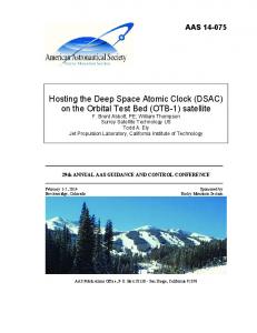
Fig. 1. The DSAC payload integrated onto OTB’s middeck payload bay.

the NASA Space Communications and Navigation Directorate (SCAN). The authors are with the Jet Propulsion Laboratory, California Institute of Technology, Pasadena CA 91109 USA (e-mail: [email protected]).

0885-3010 (c) 2018 IEEE. Personal use is permitted, but republication/redistribution requires IEEE permission. See http://www.ieee.org/publications_standards/publications/rights/index.html for more information.


2

a Frequency Electronics, Inc. (FEI) USO, a Moog TriG Global Positioning System (GPS) receiver, and GPS choke ring antenna that is hosted onboard General Atomics’ Orbital Test Bed (OTB) spacecraft. DSAC is a technology demonstrator, as such, the focus during its development has been on maturing the mercury ion trap clock technology, and not with achieving the smallest size, weight, and power (SWaP). Nonetheless, DSAC SWaP is modest, at approximately 17 l, 16 kg, and 50 W. Over the course of DSAC’ development the project has identified numerous improvements that could be made to significantly reduce these values further for an operational version. Fig. 1 shows the DSAC payload integrated into OTB’s mid-deck payload bay. OTB is one of many spacecraft missions manifested on the US Air Force’s Space Technology Program 2 Falcon Heavy launch, currently scheduled for Summer 2018. OTB will be in a 720 km, circular orbit with the GPS choke ring antenna oriented in the zenith direction. This allows for a continuous view of the GPS constellation and collection of one-way pseudo-range and phase data using the DSAC payload’s GPS receiver with DSAC as its external reference. This data, coupled with the available International GNSS Service GPS orbit and clock products, will enable the mission to validate DSAC’s performance and utility for one-way based navigation. After the mission is complete, the mercury-ion space clock technology readiness level (TRL) will mature to level 7, and attention would shift towards infusion into a planetary science mission with development focused on lifetime maturation, SWaP reduction, and other mission specific implementation details. Details of how the DSAC TDM is to be executed and the expected results are documented in [3]. II. DSAC ION CLOCK The DSAC ion clock has been described in detail in [4], and Magnetic Subsystem

Microwave / LO Subsystem Synthesizer

DSAC USO

Ion Subsystem

Ion Trap/Vacuum Tube Subsystem

Ion Trap Drive Electronics

40.5 GHz Synthesizer

User Output Synthesizer

UV source

UV detection

0.1 s resolution

Clock Controller

Clock cycle ~ 20 status monitors

UV Light Subsystem

Payload Interface

Power System

20.456 MHz Output (to GPS Rcv.)

Fig. 2. The DSAC system block diagram.

the prototype physics package (developed under prior NASA funding and advanced in the DSAC program) is described with more detail in [5], [6]. Here we summarize what was published there and give an update on characteristics of the actual clock that will be flown. A block diagram for the DSAC system is shown in Fig. 2. The basic components are the ion subsystem, which includes the quadrupole and multi-pole ion traps and the vacuum tube in which they are inserted as well as the trap drive radio frequency

(RF) electronics; the ultra-violet (UV) light subsystem, which includes the UV light source, optics, and UV detection photomultiplier tube (PMT); the microwave/local oscillator (LO) subsystem, which includes the USO, a tunable 40.5x GHz synthesizer to drive the mercury ion clock transition, and a user output synthesizer; the FPGA-based clock controller, and the power system. The DSAC payload also includes a GPS receiver (not shown in Fig. 2) that will be used to verify DSAC’s longterm stability performance in-space. A. DSAC Ion Clock Systematic Sensitivities Space clocks are often subjected to a much harsher environment than laboratory clocks. For the DSAC TDM clock, the most important environmental sensitivities are magnetic and thermal variations. For instance, the magnetic field in one orbit can vary up to almost 10-4 tesla (for a polar Earth orbit) and can be 10 times greater than that in Jovian orbit [7]. Even inside a spacecraft in orbit around the Earth, temperatures may vary by several degrees over an orbit. It is therefore critical to have accurate knowledge of the clock’s environmental sensitivities so that the impact of variations in the environment can be determined. It is possible to operate the DSAC clock by either shuttling ions between the quadrupole trap and the multi-pole trap (MP mode) or operating entirely in the simpler quadrupole trap (QP mode). Since the environmental sensitivities in each of these modes can be different, in what follows we describe the magnetic and thermal sensitivities for both modes of operation. Space qualification environmental tests performed on the DSAC clock are described in [4]. Here we focus on environmental sensitivities derived from additional laboratory measurements. The radiation sensitivity of the DSAC demonstration clock has not been measured. 1) Magnetic The DSAC magnetic subsystem consists of 3 mu-metal magnetic shields and a bias field coil. Two inner shields closely surround the vacuum tube (trap region) while a third outer shield is a box around the entire instrument (including most electronics). The coil used to define the clock quantization axis is inside the inner shields with its axis perpendicular to the trap axis. The longest shield dimension is along the trap axis so this is also the weakest shielding direction. The coil is oriented with its field in the strongest shielding direction so that external variations in the field entering in the weakest shielding direction only add to the overall field in quadrature, thereby reducing sensitivity to variations in this direction. Sensitivity to external fields were measured in all three directions using three Helmholtz coil pairs that provide a 2 gauss (2 ´ 10-4 tesla) peak to peak variation in each direction. All magnetic field measurements were static and refer to the sensitivity of the ion resonance frequency: each step in the magnetic field variation was held for 8 hours to facilitate averaging, however the results are applicable to orbital variations in the external field that will vary slowly at the orbital period of about 98 minutes. Dynamic magnetic sensitivities due to the LO or synthesizer are described in [9]. In MP mode, the weakest shielding direction has a sensitivity of 1.5(1.3) ´ 10-15/gauss. All others are 8 hours allowing the entire clock to reach thermal equilibrium. However, in orbit the 4hour thermal time constant of the instrument suppresses thermal variations experienced by the ions by a factor of 10 when they occur at the orbital period. While it is possible for the clock to be sensitive to thermal gradients, and that these would be expected for temperatures varying with a 98-minute period and with a thermal equilibrium time constant of 4 hours, here we simply report the overall measured reduction in sensitivity to such variations by a factor of 10 and note that this is what one would expect if the gradients are not too large. Thus, a typical orbital variation in temperature at the baseplate of 10°C corresponds to only 1.0°C variation at the ions. This corresponds to a peak-to-peak effect in MP mode of AMP = 1 ´ 10-14 and in QP mode of AQP < 2.2 ´ 10-14. In MP mode this will manifest itself in the Allan deviation as a 0.36 * AMP = 3.6 ´ 1015 peak at 0.37 ´ 98 minutes or about 2200 seconds [10]. In QP mode the Allan deviation peak will be < 8 ´ 10-15. Both of these are comparable to the expected 6 ´ 10-15 unperturbed Allan deviation of the clock at that averaging time and so will have only a minor impact on overall clock performance. Variations in clock frequency due to temperature effects in other orbits would need to be calculated for those orbits using the overall temperature sensitivity and thermal time constant given above. The clock electronics have been designed to have sensitivities less than that of the ions. For instance, the current source for the clock bias field coil has a temperature sensitivity of < 10 ppm/°C, which corresponds to < 1 ´ 10-15/°C (i.e. < 5 ´ 10-16 in the above example). 3) Other Systematic Effects The other primary systematic effects of this technology are decoupled, to first order, from the environment and are smaller than the thermal and magnetic effects. They have been well

characterized elsewhere [11] and remain the same or similar for the DSAC clock. These include background gas shifts [12], [13] and the ion-number–dependent second-order Doppler shift [14].

Fig. 3. Allan deviation of the DSAC ion clock operating in MP mode and compared to a hydrogen maser showing a short-term stability of 3x10-13/t1/2. Numbers next to each point in the Allan deviation indicate the number of averages associated with a given point.

B. DSAC Clock Capability: MP Mode The DSAC clock can operate with ions either in the QP or MP traps, however it was optimized for operation in the latter. As a result, the quantization axis in the QP is not as well defined and the coherence time for the clock transition there is limited currently to 2 seconds, which is the Rabi time used in that mode. In contrast, the coherence time in the MP trap is 4-6 seconds. The longer possible Rabi time results in a larger atomic line Q and a better short-term stability [4], [15] as shown in eq. (1): 𝜎𝜎"# (𝜏𝜏) =

1 𝑇𝑇 0 2; 𝜋𝜋𝜋𝜋 × SNR 𝜏𝜏

(1)

SNR = 𝑆𝑆5678 ⁄9𝑆𝑆5678 + 𝐵𝐵 .

(2) In Eq. (1), the Allan deviation 𝜎𝜎"# on the averaging time t is a function of Q, the clock cycle time 𝑇𝑇2 , the signal-to-noise ratio SNR, and 𝜏𝜏. In Eq. (2), the signal-to-noise ratio (SNR) is a function of the half-maximum point of the signal size measurement 𝑆𝑆5678 , and the amount of the background light that is not contributing to the signal measurement B. To get a better picture of the capability of this technology, Fig. 3 shows the Allan deviation of the clock operating in MP mode compared to a hydrogen maser. It is important to stress that the degradation in short-term stability due to operation in QP mode (shown in Fig. 4) is not inherent to that mode. A clock optimized for QP operation could be made to have as good or better short-term performance compared to that in MP mode. The primary fundamental advantage of MP mode is long-term stability at the 1 ´ 10-16/day level or below [14], [16]. C. Flight Operations: QP Mode After about 1 year of operation on the ground it was discovered that the amount of neon buffer gas that was loaded into the sealed vacuum tube of the DSAC clock (neon is used



4

to thermalize the trapped ions) had partially depleted. The mechanism by which the depletion had occurred is now understood to be neon ionization and subsequent implantation into surrounding surfaces. However due to schedule and resource limitations it was not possible to implement the required change for the DSAC demonstration unit. The shuttling of ions between the QP and MP traps is particularly sensitive to the level of neon present, thus MP mode operability is far more sensitive than QP mode to the buffer gas pressure. With the depletion of some of the neon, it was no longer feasible to operate in MP mode in the flight demonstration clock. However, QP mode remains viable and the lifetime for operation in this mode due to the current rate of neon depletion is much greater than the mission life, so long-term operation of the clock in space will be in QP mode. 1) Allan Deviation in QP Mode Fig. 4 shows the Allan deviation of the DSAC clock operating in QP mode for averaging intervals longer than 100 seconds compared to a hydrogen maser. The short-term stability is 5 ´ 10-13/t1/2 and the stability at one day is < 4 ´ 10-15. There is no drift removal in this data.

Fig. 4. Allan deviation of the DSAC clock for averaging intervals longer than 100 seconds while operating in QP mode.

It is important to stress that the degradation in short-term stability due to operation in QP mode (shown in Fig. 4) is not inherent to that mode. A clock optimized for QP operation could be made to have as good or better short-term performance compared to that in MP mode. The primary fundamental advantage of MP mode is long term stability at the 1x10-16/day level or below [14], [16]. Fig. 5 shows a comparison between typical DSN H-maser performance and DSAC performance in QP mode. The Allan deviation corresponding to the best SNR*Q product achieved in QP mode with a JPL ion clock is shown as the dashed black line in the graph suggesting that as the DSAC QP design is optimized, additional stability improvements can be expected. Furthermore, a significant advantage of QP-only clock operation is that its design is highly amenable to miniaturization. While this performance level satisfies DSAC requirements, it should not be taken as fully representative of the technology for reasons mentioned above. JPL trapped ion clocks operating in QP mode with a high performance local oscillator have demonstrated stabilities of 3

´ 10-14 at one second and < 1 ´ 10-15 at a day [17], [18]. Furthermore, a significant advantage of QP-only clock operation is that its design is highly amenable to miniaturization. 2) Comparison with Deep Space Network Maser Performance As described in this paper, one application of the DSAC clock is to replace two-way navigation, referenced to a hydrogen maser at each DSN site, with one-way navigation referenced to a DSAC clock located on a satellite. For comparison, Fig. 5 shows the performance of current hydrogen masers in the DSN. Even though there is a stability reduction between approximately 100 and 10,000 seconds in this particular QP trap implementation relative to the DSN H-maser, it retains a white frequency noise characteristic with little to no drift. Relative to a USO that would exhibit a frequency drift and a random walk in frequency beginning in the 1 – 100 second integration time, DSAC provides excellent stability that would introduce negligible noise to a deep space radiometric measurement (see Section III).

Fig. 5. Allan deviation of pairwise DSN hydrogen maser data (red). Typical single-maser performance observed in the DSN is 2 ´ 10-13 at one second and a drift of 2 ´ 10-15/day. Best performance observed is 1 ´ 10-13 at one second and 2 ´ 10-16/day. The >100 second Allan deviation for the current DSAC clock operating in QP mode is shown for comparison (blue) as is the best Allan deviation for a JPL clock optimized to operate in QP mode (dashed black).

III. DSAC’S BENEFITS TO NAVIGATION AND SCIENCE In today’s two-way navigation architecture, the DSN tracks a user spacecraft and then a ground-based team performs navigation. Relative to this, one-way tracking and navigation with an onboard atomic clock such as DSAC could deliver more data with better accuracy, encourage development of navigation infrastructure and flight system components to fully utilize the one-way tracking, and become a key step towards implementing autonomous radio navigation. Some specific ways that a one-way deep space tracking architecture improves upon the existing two-way architecture include: 1. One-way radiometric tracking enables use of the existing DSN Ka-band downlink capability available at all DSN antennas for tracking with almost an order of magnitude improvement in Doppler measurement precision over Xband. It should be noted that currently the DSN supports uplink Ka-band transmissions at only one antenna (DSS25), so DSAC enables full Ka-band tracking with the



5

2.

3.

4.

5.

existing DSN infrastructure, while two-way is currently a X/Ka-band hybrid with the exception of this one antenna. One-way radio tracking enables use of the existing DSN Multiple Spacecraft Per Aperture (MSPA) capability at destinations such as Mars. This yields a significant increase in tracking relative to standard two-way schedules, sometimes doubling it. One-way radio tracking can utilize the full view period of an antenna whereas two-way tracking time reduces this period by the round trip light time. At Jupiter, this can yield a 10–16% increase in tracking time, at Saturn it grows to 19–27%, and so on. One-way radiometric tracking enables use of the greater SNR of uplink signals for tracking onboard by a spacecraft receiver using low gain antennas (LGA) (use of LGAs is precluded in two-way signals due to a lower downlink SNR). As spacecraft have LGA antennas mounted on most spacecraft faces for emergency communications, radio tracking becomes nearly independent of attitude thus freeing the spacecraft from pointing to Earth for tracking and/or having the need to use a gimbaled high gain antenna for tracking. Furthermore, the spacecraft can maintain its operational attitude without interruption; thus, removing this constraint can increase science data collection. One-way radiometric tracking on a DSN uplink using a spacecraft receiver enables real-time autonomous radio navigation that, when coupled with optical navigation, provides for a robust absolute and relative navigation system.

These improvements in tracking can be applied to future missions being contemplated. Clearly, a Mars orbiter that couples the above Ka-band and MSPA capabilities (see Section VI) would benefit in both navigation and gravity science return. Studies of Europa flyby mission gravity science have shown that one-way tracking on the uplink using low gain antennas could yield a robust solution for tidal gravity effects producing more usable data than many scenarios with two-way tracking. For Mars approach, DSAC enabled one-way tracking on an uplink coupled with an onboard guidance, navigation, and control (GNC) system makes it possible to conduct autonomous operations and significantly enhance Mars atmosphere entry performance and safety (see Section V). Essentially, many mission concepts would benefit from using DSAC to improve navigation and simplify onboard timekeeping operations. A thorough discussion of some these examples have been documented in [1], [19], [20]. In this paper, the focus is more tutorial in nature and describes how one-way radio data can be used to determine spacecraft trajectories, associated model parameters (in particular gravity field information), and how clock quality affects their solutions. To illustrate this, two case studies are presented. The first examines radiometric data design and the role DSAC can have with enabling radio-based deep space autonomous navigation. The second is on how DSAC could benefit gravity determination at Mars when taking advantage of MSPA.

IV. ONE-WAY RADIOMETRIC MEASUREMENT MODELS Determining an accurate spacecraft trajectory requires several characteristic features from the measurement data: accuracy, precision, diversity, and density. For one-way data, a stable and accurate clock plays a critical role with the first two items – accuracy and precision. Diversity and density, while also impacted by onboard clock stability and accuracy, rely more on the characteristics of the trajectory and radio tracking sources. Other key factors relate to model uncertainties and their associated stochastic behavior. All of these issues will be explored when using DSAC as part of an autonomous navigation system, but to begin, we consider the model for several one-way radiometric measurement types. For those interested in a general primer on radiometric tracking see Thornton [2]. A one-way phase measurement Φ(𝑡𝑡) is a measure of the difference of two clock signals (called the beat signal and denoted as Δ𝜙𝜙(𝑡𝑡)) with one being the phase of a received radio transmission and the other being the phase of a locally generated signal within the radio receiver. Without loss of generality, all of the radiometric models considered in this paper are for one-way data types that originate from a radio source (ground station, or other satellite) and are received onboard the spacecraft of interest. As will be seen, this implies that the spacecraft clock (DSAC in the present case) participates in formulating the measurement and ‘tagging’ its associated time. Two-way radiometric models are similar, but distinct. Receiver R’s beat phase of Δ𝜙𝜙(𝑡𝑡) at the ideal time t is formed as the difference of the transmitted phase 𝜙𝜙B from transmitter T and the receiver’s reference phase 𝜙𝜙C and takes the form Δ𝜙𝜙(𝑡𝑡) = 𝜙𝜙B (𝑡𝑡 − 𝜏𝜏) − 𝑃𝑃𝑃𝑃(𝑡𝑡) − 𝜙𝜙C (𝑡𝑡) (3) = −𝑓𝑓B 𝜏𝜏 − 𝑓𝑓B [𝑥𝑥C (𝑡𝑡) − 𝑥𝑥B (𝑡𝑡 − 𝜏𝜏)] − 𝑃𝑃𝑃𝑃(𝑡𝑡), where 𝑃𝑃𝑃𝑃(𝑡𝑡) represents the ‘phase wind-up’ that results from the relative orientation changes between the receiving antenna and the transmitting antenna, 𝑓𝑓B represents the transmission frequency (to simplify the discussion, any frequency bias that might exist with a mismatch between transmission frequency 𝑓𝑓B and the receiver frequency 𝑓𝑓C has been set to zero). A clock’s time deviation 𝑥𝑥 from ideal time t is related to its phase using 𝜙𝜙 = 𝑓𝑓 × (𝑡𝑡 − 𝑥𝑥); thus, 𝑥𝑥C is defined as the receiver clock’s time deviation, and 𝑥𝑥B is the transmitter clock’s time deviation. The quantity 𝜏𝜏 is the one-way light time delay from the phase center of the transmitting antenna to the phase center of the receiving antenna and is defined as 𝜏𝜏 ≜ 𝑡𝑡C − 𝑡𝑡B = 𝑡𝑡 − 𝑡𝑡B , (4) noting that 𝑡𝑡 ≜ 𝑡𝑡C . It includes the geometric path length Δ𝑟𝑟(𝑡𝑡) as well as delays that change the path length of the signal from other effects including ionosphere 𝐼𝐼(𝑡𝑡), solar plasma 𝑆𝑆(𝑡𝑡), troposphere 𝑇𝑇(𝑡𝑡), yielding 1 (5) 𝜏𝜏(𝑡𝑡) ≅ QΔ𝑟𝑟(𝑡𝑡) − 𝐼𝐼(𝑡𝑡) − 𝑆𝑆(𝑡𝑡) + 𝑇𝑇(𝑡𝑡)R, 𝑐𝑐 where, for phase observables, the ionosphere and solar plasma delays appear to ‘shorten’ the path length; thus, the minus sign (in range observables these delays will ‘lengthen’ the path length). For simplicity in this discussion, a Newtonian approximation for the geometric path length Δ𝑟𝑟(𝑡𝑡) suffices and



6

takes the form Δ𝑟𝑟(𝑡𝑡) ≜ ‖𝐫𝐫C (𝑡𝑡) − 𝐫𝐫B (𝑡𝑡 − 𝜏𝜏)‖. (6) The vectors 𝐫𝐫C and 𝐫𝐫B represent the position of receiving antenna’s phase center and transmitting antenna’s phase center, respectively. Note that this is a generic model and the presence of the ionosphere, solar plasma, and troposphere delays are dependent on whether the signal transits through the respective media. Their computation is also dependent on the appropriate time of transit; thus, an uplink signal from the Earth to a spacecraft receiver would evaluate the ionosphere and troposphere transit at the time 𝑡𝑡 − 𝜏𝜏. For the purposes of this discussion, the functional representation of these delays on t is sufficient, where a more specific calculation must be made at the appropriate time and/or functional dependency on environment parameters will be substituted. A receiver measuring the beat phase given in Eq. (3) will add instrument delays, noise, potentially multipath effects, and introduce an integer ambiguity representing the number of complete cycles that have occurred since the signal left the transmitter. These considerations result in the following oneway phase measurement model (converted into units of length): 𝑐𝑐 Δ𝜙𝜙(𝑡𝑡) 𝑓𝑓B = Δ𝑟𝑟(𝑡𝑡) + 𝑐𝑐[𝑥𝑥C (𝑡𝑡) − 𝑥𝑥B (𝑡𝑡 − 𝜏𝜏)] − 𝐼𝐼(𝑡𝑡) − 𝑆𝑆(𝑡𝑡) + 𝑇𝑇(𝑡𝑡) + 𝑃𝑃𝑃𝑃(𝑡𝑡) + 𝑀𝑀V (𝑡𝑡) + 𝑏𝑏CV (𝑡𝑡) + 𝑏𝑏BV − 𝑁𝑁 + 𝑣𝑣(𝑡𝑡),

Φ(𝑡𝑡)≜ −

(7)

where 𝑀𝑀V (𝑡𝑡) is the error due to multipath effects, 𝑏𝑏CV (𝑡𝑡) is the receiver delay, 𝑏𝑏BV is the transmitter delay (assumed static in this discussion, i.e., 𝑏𝑏̇BV = 0), 𝑁𝑁 is the integer phase ambiguity, and 𝑣𝑣(𝑡𝑡) is the one-way phase measurement noise. It should also be noted that the receiver records the measurement with time tag 𝐶𝐶(𝑡𝑡). With this model of one-way phase, we then formulate the average one-way Doppler (in units of range rate) as the difference of adjacent phase counts separated by the Doppler count time 𝑇𝑇 as follows: Φ(𝑡𝑡) − Φ(𝑡𝑡 − 𝑇𝑇) (8) 𝐹𝐹(𝑡𝑡) ≜ . 𝑇𝑇 Upon examination of Eq. (8), Doppler eliminates the phase ambiguity (as long as the receiver doesn’t experience cycle slips or resets over the Doppler count time) and any static transmitter and receiver bias delays that would be present in the carrier phase. Only those delays that exhibit a time variation will remain in the Doppler data. One-way ranging collected by a spacecraft receiver has a model that is very similar in form to the carrier phase model in Eq. (8), and is formally represented using 𝑅𝑅(𝑡𝑡) = 𝛥𝛥𝛥𝛥(𝑡𝑡) + 𝑐𝑐[𝑥𝑥C (𝑡𝑡) − 𝑥𝑥B (𝑡𝑡 − 𝜏𝜏)] + 𝐼𝐼(𝑡𝑡) + 𝑆𝑆(𝑡𝑡) + (9) 𝑇𝑇(𝑡𝑡) + 𝑀𝑀` (𝑡𝑡) + 𝑏𝑏C` (𝑡𝑡) + 𝑏𝑏B` + 𝜀𝜀(𝑡𝑡) where the differences between the range expression in Eq. (9) versus the phase in Eq. (7) include sign changes on the ionosphere and solar plasma delays, different receiver delays 𝑏𝑏C` (𝑡𝑡) (including temperature sensitivities), multipath 𝑀𝑀` (𝑡𝑡), measurement noise 𝜀𝜀(𝑡𝑡), and no phase ambiguity. Examination of the phase and range models in Eqs. (7) and (9), respectively, reveals that the receiver clock phase error 𝑥𝑥C (𝑡𝑡) appears directly and is multiplied by the speed of light c. Hence, even the smallest clock error manifests itself in a

significant way. Consider that for the typical deep space mission, Doppler measurement noise at X-band is less than 0.1 mm/sec on a 60 second count time, the equivalent AD on this integration time is 2.4 ´ 10-13. Additionally, as the count time increases the Doppler measurement noise strength decreases and, ideally, the impact of onboard clock errors would also decrease. On short time scales, DSAC’s output is similar to its paired USO with AD near 1 ´ 10-13, and on longer time scales yields a stabilized frequency output with AD of 2 ´ 10-15 at one day (with a demonstrated potential using the DSAC technology to achieve < 1 ´ 10-15 at a day). It is useful to examine the individual clock error contributions to one-way Doppler further. The expression that includes the receiver and transmitter clock effects present in the Doppler measurement model of Eq. (8) can be expressed as 𝑐𝑐 b𝑥𝑥 (𝑡𝑡)−𝑥𝑥C (𝑡𝑡 − 𝑇𝑇) − 𝑥𝑥B Q𝑡𝑡 − 𝜏𝜏(𝑡𝑡)R 𝑇𝑇 C (10) + 𝑥𝑥B Q𝑡𝑡 − 𝑇𝑇 − 𝜏𝜏(𝑡𝑡 − 𝑇𝑇)Rc. To simplify the discussion, it is assumed the transmitter’s reference (typically a hydrogen maser) is based at a DSN station in a controlled environment. For a typical 60 second Doppler count time the DSN hydrogen maser’s Allan deviation 𝜎𝜎d (60) falls below 1 ´ 10-14 (see Fig. 5) and conforms approximately to white frequency noise for integration times less than 1000 seconds; additionally, the frequency bias and drift terms are ignorable [1]. These considerations lead to a range rate error contribution of approximately 3 ´ 10-4 mm/s (using 𝜎𝜎f (𝑇𝑇) = 𝑇𝑇𝑇𝑇d (𝑇𝑇)), which is insignificant relative to a typical X-band Doppler noise at 60 seconds of 0.1 mm/s, or even 0.01 mm/s for Ka-band Doppler. Expanding the expression for the receiver frequency reference takes the form 𝑐𝑐 [𝑥𝑥 (𝑡𝑡)−𝑥𝑥C (𝑡𝑡 − 𝑇𝑇)] = 𝑐𝑐b𝑑𝑑C + 𝑎𝑎C 𝑇𝑇 + 𝜓𝜓d (𝑇𝑇)c, (11) 𝑇𝑇 C where 𝑑𝑑C is the clock rate (or fractional frequency bias), 𝑎𝑎C is the clock acceleration (fractional frequency drift or aging), and 𝜓𝜓d (𝑇𝑇) is a stochastic increment of the clock’s fractional frequency instability and is related to the clock’s phase instability via 𝜓𝜓f (𝑇𝑇) = 𝑇𝑇𝜓𝜓d (𝑇𝑇). Comparing DSAC to a USO, DSAC’s fractional frequency drift term is insignificant at < 3 ´ 10-15/day, whereas a USO’s drift term is on the order of a few parts in 10-11/day and subject to discontinuous shifts which impact 𝑑𝑑C . Furthermore, a USO’s stochastic instability is a frequency random walk with an Allan deviation that grows unbounded as ∝ 9𝑡𝑡 − 𝑡𝑡k, while DSAC’s instability is white frequency noise that diminishes with time as ∝ 1⁄9𝑡𝑡 − 𝑡𝑡k. A navigation filter processing one-way Doppler from a USO accounts for these effects via estimating them and, given that a DSN pass could have gaps of hours to days, would need to reestimate the USO’s {𝑑𝑑C , 𝑎𝑎C } pair anew (i.e., wide open a priori uncertainties) on every pass. Whereas, with the expected DSAC performance, DSAC’s contribution to the range rate error would be white frequency noise with equivalent range rate error < 0.03 mm/s at 60 seconds, and the navigation filter would not necessarily account for DSAC drift in its estimation state. In other words, DSAC based one-way Doppler can be treated in a similar fashion to its two-way counterpart – a key reason DSAC



7

has been developed. With one-way tracking, at least one end of the link is at a spacecraft (both ends for spacecraft-to-spacecraft tracking), and the environmental conditions at the spacecraft (such as voltage, temperature, magnetic fields, radiation) are often more difficult to control, as compared to the DSN, and have a greater potential to impact the radiometric tracking function of the receiver and reference pair. DSAC represents a leap forward in minimizing environmental sensitivity of the frequency and timing reference by orders of magnitude over its USO counterparts. However, to take full advantage of this stability requires the receiving radio to also be relatively insensitive to environments [20]. V. USING DSAC FOR AUTONOMOUS NAVIGATION: A MARS ENTRY CASE STUDY Navigating in deep space is very different from typical terrestrial applications where the presence of global navigation satellite systems (GNSSs), such as GPS or Galileo, are ubiquitous. These systems provide a rich data environment for terrestrial positioning or low Earth orbit determination. There are typically a sufficient number of GNSS satellites in view that a position or orbit estimate can be determined uniquely with each set of measurements that a receiver collects at any given time. These types of solutions are kinematic, relying only on the geometric diversity and known information about the GNSS transmitter locations and clocks with results that are accurate to meters, and sometimes centimeters. In contrast, deep space navigation is characterized as having sparse data that is rarely sufficient to produce a kinematic position and velocity fix. Fundamentally, the accuracy of the orbit determination process relies on the geometric diversity introduced by measurements that are collected over time, and fidelity of the dynamic and measurement models required to compute the nominal measurements, trajectories, and associated partials. Data collected over time implies that time-dependent effects, whether deterministic or stochastic, are more significant to the solution accuracy of a position (and or velocity) than is the case for solutions that can be determined kinematically. As a specific example, in GPS-based orbit determination of a low Earth orbiting satellite, the clock is determined simultaneous with the orbit without regard to the characteristics of the onboard clock driving the GPS receiver. In deep space cruise navigation, range and Doppler data are collected from a single Deep Space Network antenna over a pass typically lasting 8 hours or more, with the next pass several days to a week later. A batch of passes over weeks to months are then used to solve for the trajectory. In this scenario, if one-way radiometric data were used, then the characteristics of the clock would be critical to the ultimate solution accuracy that is achievable. Furthermore, modeling errors of the spacecraft’s dynamics (such as the spacecraft’s solar reflective properties, outgassing, thruster accelerations, and others), or unknown measurement effects such as those noted in Eq. (8) or Eq. (9) could have a significant impact on the solution accuracy. Examples of high fidelity spacecraft modeling used for ground-based deep spacecraft navigation in recent missions to Mars can be found in [21]–[25]. To illustrate the impact of transitioning deep space navigation from two-way radiometric tracking using standard groundbased processing techniques towards one-way onboard

radiometric tracking and processing, a representative example will be examined for the approach navigation of a Mars lander in the final weeks prior to entry into the Martian atmosphere. Continuous DSN coverage is usually provided for a Mars’ approaching spacecraft in the last 30 - 45 days prior to entry with a typical pass on each antenna lasting about 8 hours, and a measurement frequency of 60 seconds for two-way Doppler and 180 seconds for range. The models and associated modeling errors utilized are similar to those of NASA’s InSight Mars lander as documented in [26]. In particular, the filter modeling details for processing standard two-way DSN range and Doppler data is provided in [26], and has been used in the present study. These models assume availability of high fidelity model calibration data for Earth atmosphere effects, Earth orientation, detailed spacecraft modeling for thrusts including reaction control system effects. Simulation results of the RSS position errors and uncertainties for the lander’s approach trajectory in the final 45 days prior to entry using these high-fidelity models, calibration data, and tracking from two-way range and Doppler are presented in Fig. 6. Two-way range and Doppler with high fidelity models and calibrations

Fig 6. RSS position errors/uncertainties for Mars approach navigation using (top) two-way Doppler and range using full fidelity models and all available calibration data, and (bottom) are the two-way tracking passes to the DSN stations at Goldstone, USA (DSS-15), Madrid, Spain (DSS-45), and Canberra, Australia (DSS-65).

The red curves in Fig 6. (labeled sigma) represent the 1sigma uncertainties produced by the navigation filter, and the blue curves (labeled error) represent the filter solution error. Employing an ergodic process assumption, a useful heuristic for a properly tuned filter is to have the solution errors fall within the 1-sigma uncertainty bounds at least 68% of the time. The bottom plot in Fig. 6 depicts the two-way tracking passes between the spacecraft and the lander. Note that the uncertainties begin with an initial filter transient, and then settle to somewhere in the 1 – 10 km range. As the lander nears entry, Mars’s gravity becomes more significant and yields a reduction in the solution’s uncertainty during the final hours – less than 100 m at Mars’ entry (~1080 hrs in elapsed time). However, for ground-based navigation, the trajectory solutions in the final hours before entry using all the available data are never known



8

in sufficient time to be uploaded to the spacecraft to be useful during atmospheric entry and landing. Typical ground-based navigation cuts data tracking off at 6 hrs prior to entry to determine a solution and upload it as the final entry state to the spacecraft. In this example, that results in a trajectory knowledge error of ~3 km (1-sigma) at atmospheric entry. Other example Mars missions, such as the Mars Science Laboratory, have achieved better ground-based, predicted position knowledge at Mars atmosphere entry via a combination of a more dynamically quiet vehicle and the addition of Delta Differenced One-Way Ranging (DDOR) – a standard practice for Mars’ missions today – but even in this case the predicted position knowledge at the top of the atmosphere remained around one kilometer [33]. Now we consider replacing the ground-based two-way tracking with one-way tracking collected onboard and using DSAC as the spacecraft’s time and frequency reference. First, we retain all the model fidelity and calibrations from the prior two-way example (later, we consider model reductions). The intent is to determine the impact of using one-way data as compared to two-way. Because there are now independent transmitter and receiver clocks, the navigation filter state needs to expand to include estimating any offsets between them. Fortunately, since the spacecraft clock is DSAC it is sufficient to estimate the frequency and time offsets only as biases with constrained a priori uncertainties (in the present case a 1 ´ 10-6 sec initial time offset, and 1 ´ 10-14 initial frequency offset). DSAC’s stochastic frequency effects are sufficiently small (and white frequency like) such that they do not appreciably impact the data quality. The same could not be said if the spacecraft’s local oscillator where a USO or TCXO. The Mars approach navigation results obtained when using one-way radiometric tracking are shown in Fig. 7. It is clear that the qualitative results are unchanged relative to their two-way counterparts, and, moreover, the quantitative differences are small enough that they do not affect the results in any meaningful way. It should be noted that this result relies on the ability of the spacecraft clock to remain stable and free of any large excursions or unmodeled drifts after an initial calibration, as would be expected with a clock like DSAC. This result also supports the claim that one-way radiometric data with DSAC can be treated in a manner similar to two-way for navigation. We now examine the impact of moving the orbit determination process to an onboard, autonomous navigation system where it will be necessary to account for additional complexities including: 1. High-fidelity, ground-based calibration data not being available, 2. Limited onboard computing resources, 3. Automating the assessment of trajectory solution validity where any mismodeling that leads to an incorrect trajectory solution could have a significant effect on mission safety. Even with these complexities present, autonomous navigation using JPL’s AutoNav software system has already been a critical technology for several deep space missions, including

Deep Space 1, Stardust, and Deep Impact [27]. These missions’ autonomous navigation was conducted using passive optical imaging of nearby bodies with an onboard camera system. Optical data provides strong angular information about a spacecraft’s ‘plane-of-sky’ relationship to the object being imaged. Range (or ‘line-of-sight’) information, orthogonal to the plane-of-sky, is more difficult to determine from optical data due to the slow rate of angular change seen with observed bodies. A more direct measure of line-of-sight is obtained with radiometric tracking of range and Doppler. These complement the optical data such that, when combined, yield a more robust solution for a spacecraft’s trajectory. With DSAC, operationally accurate and reliable one-way radiometric signals sent from radio beacons (i.e., DSN antennas or other spacecraft) and measured using a spacecraft’s radio receiver enables the fusion of these two data types into a more capable and robust autonomous deep space navigation capability than is available today. A robust onboard navigation system needs to maximize selfreliance. Measurement model calibration data that requires significant ground support, or cannot be obtained in real-time, would limit that measurement’s utility to support autonomous navigation. Specifically, ground-based two-way radiometric data requires atmospheric media (troposphere and ionosphere) delay data, high precision Earth orientation data, and range bias data to support high fidelity orbit determination. One-way range and Doppler with DSAC and full fidelity models and calibrations

Fig 7. RSS position errors/uncertainties for Mars approach navigation using (top) one-way Doppler and range using full fidelity models and all available calibration data, and (bottom) are the one-way tracking passes with the data being collected on the spacecraft (named ‘otto’).

Charged particle effects can be one of the most significant error sources in radio-based approach navigation to a planetary body such as Mars [28]. It is possible to eliminate the need to calibrate for these effects (i.e., ionosphere and/or solar plasma) via a judicious combination of the range in Eq. (9) and phase in Eq. (7). The derived data type, referred to as charged-particle– free (CPF) phase, can be obtained using 𝑅𝑅(𝑡𝑡) + Φ(𝑡𝑡) (12) Φnop (𝑡𝑡) ≜ , 2



9

where the resulting model takes the form Φnop (𝑡𝑡) = Δ𝑟𝑟(𝑡𝑡) + 𝑐𝑐[𝑥𝑥C (𝑡𝑡) − 𝑥𝑥B (𝑡𝑡 − 𝜏𝜏)] + 𝑇𝑇(𝑡𝑡) + 𝑃𝑃𝑃𝑃(𝑡𝑡)⁄2 + 〈𝑀𝑀(𝑡𝑡)〉 + 〈𝑏𝑏C (𝑡𝑡)〉 + 〈𝑏𝑏B 〉 − (13) 𝑁𝑁⁄2 + Q𝑣𝑣(𝑡𝑡) + 𝜀𝜀(𝑡𝑡)R⁄2. Note that neither charged-particle delays from the ionosphere nor solar corona plasma effects are present. This eliminates the need to calibrate for these at the expense of an increased overall noise relative to the phase by itself (DSN-based range measurement noise typically is 1 to 3 m (1-s) while the phase noise is 5 mm (1-s)). More importantly, the measurement noise is white while charged-particle stochastic effects are correlated and have difficult-to-model temporal effects (such as the day/night cycle). Simpler stochastic modeling yields a more robust filter for obtaining convergent and correct trajectory solutions. The effects of the phase ambiguity term can be minimized to the level of the range error via using the range measurement value at the beginning of a pass to calibrate for the ambiguity. This has the subtle effect of ‘pushing’ range errors (including charged-particle effects) into the range bias, but these are observable for each pass of data. A conservative bound for the range bias uncertainty (including charge particle delays at X-band) is 3 m (1-sigma). Unlike ionosphere and solar plasma effects, troposphere daily effects (on the order of a ~ 5 cm delay) are readily dealt with using an appropriately tuned stochastic model or via increasing the measurement uncertainty of the CPF phase data. What remains is a seasonal troposphere delay that can be calibrated using a compact model in the onboard orbit determination models [29]. The remaining real-time model considerations are the high precision Earth orientation models and their impact on an onboard implementation when daily calibrations for, primarily, Earth pole motion and UT1 time drift are not present. Kalarus, et. al. [30] have thoroughly documented the characteristics of the high precision Earth orientation calibrations available from the International Earth Rotation Systems Service (IERS) for reconstruction and prediction (for periods of up to 500 days). They find that both pole motion and UT1 predict errors grow unbounded to levels near 80 mas and 80 ms, respectively, after 500 days. A real time, onboard navigation system will have to utilize predictive models for months at a time (depending on the specific mission context). To model this effect, historical data including actuals for the truth simulation and predicts for the onboard nominals have been used in the simulation. It should be noted that the arrival of multiple measurements, at differing times, and with gaps requires modifications to the filtering algorithms in significant ways as documented in [31]. This reference also describes the proper way to model a clock and its associated stochastic processes in the resultant filter model. Utilizing the preceding measurement model simplifications, autonomous navigation when processing one-way CPF phase with DSAC as the reference is illustrated in Fig. 8 for the Mars approach case. Note that the dynamic spacecraft models are the same as before - a next step is to study the effects of model fidelity reduction for the spacecraft to a more suitable onboard

model. Inspecting Fig. 8 and Fig. 7 indicates that the effect of the model simplifications increased the trajectory uncertainty by about ten times with an upper bound near 40 km. However, the uncertainty drop during the final hours is still present and the atmospheric entry knowledge remains better than 100 m, similar to the full fidelity modeling exhibited in Fig. 7. Unlike the two-way ground processing with predicts, the entry knowledge would be onboard and now available in real-time so that it could be utilized by the flight system to improve guidance during atmospheric flight and landing. One-way CPF phase with no near real-time calibration data

Fig 8. RSS position errors/uncertainties for Mars approach navigation using CPF phase with no daily troposphere calibration, no ionosphere calibration, and scaled ambiguity resolution.

To improve upon these results and enhance the solution robustness, adding onboard optical images to the CPF phase observables is investigated. The optical image simulations are of Phobos and Deimos, Mars’ moons, and assume a camera system consisting of both a gimbaled narrow-angle and wideangle camera. A description of the proposed camera system can be found in Ref. [32]. Because the camera is gimbaled it is possible to have a near continuous duty cycle, in the present case an image is taken every 10 minutes. Preliminary results for this case are shown in Fig. 9. It should be noted that, unlike the prior results, spacecraft dynamic errors have not been simulated and included (only the measurement and calibrations errors are present). However, the filter model remains the same as was used to obtain the prior results and still accounts for random/stochastic effects from maneuver errors, solar pressure errors, and reaction control system errors. Hence, the solution uncertainties (the red curve) remain representative of the combined CPF phase/optical solution accuracy, even though the simulated errors are optimistic. The most notable result is the combination of the two data types reduces the overall trajectory uncertainties by over an order of magnitude. This is a key reason to include both the radio and optical data types in the first place, as the combined solutions are more accurate than either by themselves. To fully assess the ability to execute autonomous deep space



10

One-way CPF phase and optical images with no near real-time calibration data

Fig 9. RSS position errors/uncertainties for Mars approach navigation using CPF phase and optical imagery of Phobos and Deimos. Note that the tracking schedule in the lower plot also shows the periods when the narrow-angle camera (NA) and wide-angle camera (WA) are actively taking images.

navigation using one-way CPF phase combined with optical data additional research is required, particularly in finding appropriate spacecraft model fidelity reduction that would be sufficient for a resource-limited implementation in an onboard flight computer. This is a topic of current investigation by the authors. VI. USING DSAC FOR RADIO SCIENCE: A MARS ORBITER CASE STUDY We turn our attention to an example of how DSAC could benefit orbit determination and radio science at Mars where numerous satellites, landers, and rovers require tracking and support from the DSN. What follows has been previously published in [1], and is presented here (in abbreviated form) to demonstrate DSAC’s utility for radio science and to complement the earlier discussion on navigating with DSAC autonomously. Due to the relatively high density of Martian assets, a Mars orbiter with DSAC could get more tracking time by exploiting the DSN’s Multiple Spacecraft Per Aperture (MSPA) capability and more accurate tracking via use of the DSN’s Ka-band downlink tracking capabilities. With MSPA, the DSN is able to receive and track multiple downlink signals using a single DSN antenna. Currently, each DSN antenna can track four simultaneous downlink signals, while only a single two-way link can be supported at a time. MSPA enables increased tracking of a Mars spacecraft, because it eliminates the need to ‘time share’ the uplink with other spacecraft to get two-way tracking. Furthermore, many DSN antennas support receiving a signal at the Ka-band frequency. Transmission at this higher frequency reduce charged-particle effects (both from the solar plasma and the ionosphere) by up to a factor of (𝑓𝑓t6 ⁄𝑓𝑓u )v ~19; however, because of other effects, a more conservative factor of improvement is 10. The scenario we examine is configured to mimic Mars Reconnaissance Orbiter (MRO) operational navigation and

gravity field reconstruction [34], [35]. The details of the scenario are described in [1]; of relevance to the present discussion are the typical tracking levels that are achievable with traditional two-way tracking and what is possible with one-way downlink tracking using MSPA. Traditionally, a Mars orbiter suffers two-way tracking gaps when the DSN is committed to tracking other spacecraft; a statistical assessment of the Mars Reconnaissance Orbiter (MRO) and Mars Odyssey two-way tracking schedules over a three-month period revealed that the average gap is 3 to 5 hours in duration, occurring several times per day. However, both spacecraft infrequently experience lengthy tracking gaps, approximately 8 to 10 hours in duration, a few times each month. The arrival of the Mars Atmosphere and Volatile EvolutioN (MAVEN) orbiter in late 2014 stressed this even further. Fig. 10 (top) presents a typical DSN tracking schedule of a Mars orbiter, including a 10-degree elevation mask. While the spacecraft is always geometrically visible to at least one DSN ground antenna (except for those times when Mars occults the spacecraft – typically 20 to 30 minutes per orbit as seen in Fig. 10), 10-hour tracking gaps have been inserted to represent times during which the DSN is tracking other assets. It is reasonable to assume that at any time at least one antenna is pointed toward bodies hosting multiple spacecraft, such as Mars or the Moon. For this case, the DSN’s Two−Way Tracking Schedule

Madrid

Canberra

Goldstone 0

5

10

15

20

25

30

35

40

45

5

10

15

20

25

30

35

40

45

Madrid

One−WayTracking Schedule

Canberra

Goldstone 0

Time (hr)

Fig. 10. DSN tracking schedules for simulated Mars orbiter given two-way (top) and one-way tracking (bottom)

MSPA capability may be exploited in a downlink capacity; where a DSN antenna can only perform two-way communications with one spacecraft at a time, it can receive multiple downlink signals simultaneously. In this manner, oneway downlink-only tracking data can be available continuously (excepting for occultations). This one-way continuous tracking configuration is illustrated in Fig. 10 (bottom). Doppler measurements were generated from the truth trajectory in accordance with the two-way and one-way DSN tracking schedules shown in Fig. 10. Two-way X-band Doppler measurements were generated following the two-way discontinuous tracking schedule. Two independent one-way Doppler measurement sets were simulated following the continuous tracking schedule: one-way X-band with DSAC, and one-way Ka-band with DSAC. For simplicity, Gaussian noise degradation of the measurements was performed at the traditionally utilized 0.1 mm/sec (X-band) and 0.01 mm/sec



11

Gravity Term 3−sigma Uncertainty (x1e−9)

3

2−way X 1−way X, DSAC 1−way Ka, DSAC

2

1

0

−1

−2

−3 0

10

20

30

40

50

Gravity Terms

60

70

80

90

Fig. 11: Static gravity field error (identified by standalone markers for each gravity term and tracking scenario) and associated 3σ uncertainty (identified by connecting lines – for visual clarity only – between consecutive markers of the same type) given standard two-way or one-way Doppler tracking data scenarios using X-band or Ka-band and DSAC as the onboard reference.

(Ka-band) levels. Stochastic clock noise was also incorporated into the measurements in order to reflect the stochastic clock behavior of both the DSN Frequency and Timing Subsystem (FTS) and the onboard frequency source (in the present case, DSAC). The DSN Frequency and Time System (FTS) clock noise was modeled as white frequency noise with an Allan deviation of 1 ´ 10-15 at 1000 seconds. The DSAC stochastic model includes a USO flicker floor of 1 ´ 10-13 up to 10 seconds, and then white frequency noise in accordance with performance of 1 ´ 10-15 at 1 day. In addition to using this tracking data to navigate a Mars orbiter, the data may also be utilized to reconstruct portions of the Martian static gravity field. In so doing, the improvements to reconstruction of the Martian static gravity field via DSACenabled one-way Doppler tracking as compared to traditional two-way Doppler tracking are highlighted. Several steps were taken in the simulation to closely mimic the process used for Mars gravity science. The orbiter’s truth trajectory was propagated over a 4-day span and includes the dynamic effects of a 50 ´ 50 Mars spherical harmonic gravity field. The continuous and discontinuous DSN tracking schedules shown in Fig. 10 were extended by concatenating the two-way tracking schedule presented in Fig. 10 to cover the simulations 4 – day span, and likewise for the one-way schedule. The gravity science filter, in addition to estimating the spacecraft position, velocity, solar pressure and drag scale factors, also estimated selected gravity field terms within a 40 ´ 40 field that were observable over the selected 4-day arc. For the simulated orbit and period, the observable gravity terms are given by

𝐶𝐶|k,} 𝑆𝑆|k,} 𝐶𝐶~,~| , 𝑛𝑛 = 12, … ,28 𝑆𝑆~,~| , 𝑛𝑛 = 12, … ,28 ⎫ . 𝐶𝐶~,~ , 𝑛𝑛 = 12, … ,28 𝑆𝑆~,~ , 𝑛𝑛 = 12, … ,28 ⎬ ⎨ ⎩𝐶𝐶~,~| , 𝑛𝑛 = 29, … , 32, 34, 40 𝑆𝑆~,~| , 𝑛𝑛 = 29, … , 32, 34⎭ ⎧

(14)

Fig. 11 presents the formal uncertainty (3σ) and error of the estimated Mars normalized gravity terms for each of the independently processed Doppler data sets. For brevity, the estimated gravity terms shown in Eq. (14) have simply been numbered sequentially. The DSAC-enabled one-way Doppler solutions offer a significant improvement in gravity solution quality compared to the two-way X-band Doppler solution; on average the solution uncertainty is decreased by factors of ~2 and ~12 given the X-band and Ka-band one-way Doppler data, respectively. These improvements are due primarily to the more abundant data that DSAC enables via MSPA, and, for Kaband, the reduction of charged-particle effects. VII. CONCLUSION The DSAC mission is poised to launch and test the next generation of space navigation atomic clock with an anticipated performance exceeding that of the space atomic clocks in use today. Furthermore, the DSAC mission will demonstrate the utility of the mercury ion atomic clock technology for deep space navigation and radio science. Space-worthy atomic frequency standards, such as DSAC, could be used to enhance robotic exploration via improved navigation performance and science derived from superior data quality and availability. It would also enable radio-based autonomous navigation and form part of a robust onboard navigation system that combines both radio and optical data processing.



12

[1]

[2]

[3]

[4]

[5]

[6]

[7] [8]

[9]

[10]

[11]

[12]

[13]

REFERENCES

T. A. Ely, J. Seubert, and J. Bell, “Advancing Navigation, Timing, and Science with the Deep-Space Atomic Clock,” in Space Operations: Innovations, Inventions, and Discoveries, American Institute of Aeronautics and Astronautics, Inc., 2015, pp. 105– 138. C. L. Thornton, J. S. Border, John Wiley & Sons., and Wiley InterScience (Online service), Radiometric tracking techniques for deep-space navigation. WileyInterscience, 2003. T. A. Ely, D. Murphy, J. Seubert, J. Bell, and D. Kuang, “Expected Performance of the Deep Space Atomic Clock Mission,” in AAS/AIAA Space Flight Mechanics Meeting, 2014. R. L. Tjoelker et al., “Mercury Ion Clock for a NASA Technology Demonstration Mission,” IEEE Trans. Ultrason. Ferroelectr. Freq. Control, vol. 63, no. 7, 2016. J. D. Prestage and G. L. Weaver, “Atomic Clocks and Oscillators for Deep-Space Navigation and Radio Science,” Proc. IEEE, vol. 95, no. 11, pp. 2235–2247, Nov. 2007. J. D. Prestage, Meirong Tu, S. K. Chung, and P. MacNeal, “Compact microwave mercury ion clock for space applications,” in 2008 IEEE International Frequency Control Symposium, 2008, pp. 651–654. C. A. Jones, “A dynamo model of Jupiter’s magnetic field,” Icarus, vol. 241, pp. 148–159, Oct. 2014. R. L. Tjoelker, J. D. Prestage, G. J. Dick, and L. Maleki, “Long term stability of Hg+ trapped ion frequency standards,” in 1993 IEEE International Frequency Control Symposium, 1993, pp. 132–138. R. L. Tjoelker et al., “Mercury trapped ion frequency standard for space applications,” in Proceedings of the 6th Symposium on Frequency Standards and Metrology, 2001, pp. 609–614. D. G. Enzer, W. A. Diener, D. W. Murphy, S. R. Rao, and R. L. Tjoelker, “Drifts and Environmental Disturbances in Atomic Clock Subsystems: Quantifying Local Oscillator, Control Loop, and Ion Resonance Interactions,” IEEE Trans. Ultrason. Ferroelectr. Freq. Control, vol. 64, no. 3, pp. 623– 633, Mar. 2017. E. A. Burt, S. Taghavi, J. D. Prestage, and R. L. Tjoelker, “Stability evaluation of systematic effects in a compensated multi-pole mercury trapped ion frequency standard,” in 2008 IEEE International Frequency Control Symposium, 2008, pp. 371–376. S. K. Chung, J. D. Prestage, R. L. Tjoelker, and L. Maleki, “Buffer gas experiments in mercury (Hg+) ion clock,” in Proceedings of the 2004 IEEE International Frequency Control Symposium and Exposition, 2004., 2004, pp. 130–133. L. Yi, S. Taghavi-Larigani, E. A. Burt, and R. L. Tjoelker, “Progress towards a dual-isotope trapped mercury ion atomic clock: Further studies of background gas collision shifts,” in 2012 IEEE International Frequency Control Symposium

[14]

[15]

[16]

[17]

[18]

[19]

[20]

[21]

[22] [23]

[24]

[25]

[26]

Proceedings, 2012, pp. 1–5. J. D. Prestage, R. L. Tjoelker, and L. Maleki, “Higher pole linear traps for atomic clock applications,” in Proceedings of the 1999 Joint Meeting of the European Frequency and Time Forum and the IEEE International Frequency Control Symposium (Cat. No.99CH36313), 1999, vol. 1, pp. 121–124. J. D. Prestage, R. L. Tjoelker, and L. Maleki, “Recent Developments in Microwave Ion Clocks,” in Frequency Measurement and Control, Berlin, Heidelberg: Springer Berlin Heidelberg, 2001, pp. 195–211. E. A. Burt, W. A. Diener, and R. L. Tjoelker, “A compensated multi-pole linear ion trap mercury frequency standard for ultra-stable timekeeping,” IEEE Trans. Ultrason. Ferroelectr. Freq. Control, vol. 55, no. 12, pp. 2586–2595, Dec. 2008. R. L. Tjoelker et al., “A Mercury Ion Frequency Standard Engineering Prototype for the NASA Deep Space Network,” in 1996 IEEE International Frequency Control Symposium, 1996, pp. 1073–1081. G. J. Dick, R. T. Wang, and R. L. Tjoelker, “Cryocooled sapphire oscillator with ultra-high stability,” in Proceedings of the 1998 IEEE International Frequency Control Symposium (Cat. No.98CH36165), 1998, pp. 528–533. J. Seubert and T. Ely, “Utilization of the Deep Space Atomic Clock for Europa Gravitational Tide Recovery,” in AAS/AIAA Space Flight Mechanics Meeting, 2015. T. A. Ely and J. Seubert, “One-Way Radiometric Navigation with the Deep Space Atomic Clock,” in Advances in the Astronautical Sciences Spaceflight Mechanics, Vol. 155, 2015. G. Wawrzyniak, D. Baird, E. Graat, T. McElrath, B. Portock, and M. Watkins, “Mars exploration rovers orbit determination system modeling,” J. Astronaut. Sci., vol. 54, no. 2, pp. 175–197, Jun. 2006. M. Ryne et al., “Orbit Determination for the 2007 Mars Phoenix Lander,” AIAA/AAS Astrodynamics Specialist Conference. Honolulu, Hawaii, 2008. B. M. Portock, G. Kruizinga, E. Bonfiglio, B. Raofi, and M. Ryne, “Navigation Challenges of the Mars Phoenix Lander Mission,” AIAA/AAS Astrodynamics Specialist Conference. Honolulu, Hawaii, 2008. T. J. Martin-Mur, G. L. Kruizinga, P. D. Burkhart, F. Abilleira, M. C. Wong, and J. A. Kangas, “Mars Science Laboratory Interplanetary Navigation,” J. Spacecr. Rockets, vol. 51, no. 4, pp. 1014–1028, Jul. 2014. M. Jesick, S. Demcak, B. Young, D. Jones, S. E. McCandless, and M. Schadegg, “Navigation Overview for the Mars Atmosphere and Volatile Evolution Mission,” J. Spacecr. Rockets, vol. 54, no. 1, pp. 29– 43, Jan. 2017. F. Abilleira et al., “Final Mission and Navigation Design for the 2016 Mars Insight Mission,” in Advances in the Astronautical Sciences, Vol. 158, 2016, pp. 1311–1329.



13

[27] [28]

[29]

[30]

[31]

[32]

[33]

[34] [35]

S. Bhaskaran, “Autonomous Navigation for Deep Space Missions,” in 12th International Conference on Space Operations, 2012. T. McElrath, M. Watkins, B. Portock, E. Graat, D. Baird, and G. Wawrzyniak, “Mars Exploration Rovers Orbit Determination Filter Strategy,” in AIAA/AAS Astrodynamics Specialist Conference and Exhibit, 2004. J. A. Estefan and O. J. Sovers, “A Comparative Survey of Current and Proposed Tropospheric Refraction-Delay Models for DSN Radio Metric Data Calibration,” 1994. M. Kalarus et al., “Achievements of the Earth orientation parameters prediction comparison campaign,” J. Geod., vol. 84, no. 10, pp. 587–596, Oct. 2010. T. A. Ely and J. Seubert, “Batch Sequential Estimation with Non-uniform Measurements and Non-stationary Noise,” in AAS/AIAA Astrodynamics Specialist Conference, 2017. J. R. Guinn et al., “The deep-space positioning system concept: Automating complex navigation operations beyond the earth,” in AIAA Space and Astronautics Forum and Exposition, SPACE 2016, 2016. L. D’Amario, “Mission and Navigation Design for the 2009 Mars Science Laboratory Mission,” 59th International Astronautical Congress. Glasgow, Scotland, 2008. T.-H. You et al., “Navigating Mars Reconnaissance Orbiter: Launch Through Primary Science Orbit,” in AIAA Space 2007 Conference and Exposition, 2007. M. T. Zuber, F. G. Lemoine, D. E. Smith, A. S. Konopliv, S. E. Smrekar, and S. W. Asmar, “Mars Reconnaissance Orbiter Radio Science Gravity Investigation,” J. Geophys. Res., vol. 112, no. E5, p. E05S07, May 2007.

the Jet Propulsion Laboratory, California Institute of Technology, Pasadena, CA, USA. Robert L. Tjoelker (M’98–SM’05) received degrees in architecture, mathematics, and physics from the University of Washington, and the Ph.D. degree in physics from Harvard University, in 1990. He is a DSAC clock co-investigator and Technical Group Supervisor of the Frequency and Timing Advanced Development Group with the Jet Propulsion Laboratory, California Institute of Technology, Pasadena, CA, USA.

Todd A. Ely received the Ph.D. degree in aeronautics and astronautics from Purdue University, in 1996. He is the DSAC mission principal-investigator and project manager with the Jet Propulsion Laboratory, California Institute of Technology, Pasadena, CA, USA. Eric A. Burt (M’02) received the Ph.D. degree in physics from the University of Washington, in 1995. He is a clock development physicist and the DSAC clock optimization lead with the Jet Propulsion Laboratory, California Institute of Technology, Pasadena, CA, USA. John D. Prestage (M’95) received the Ph.D. degree in physics from Yale University, in 1983. He is a DSAC clock co-investigator with the Jet Propulsion Laboratory, California Institute of Technology, Pasadena, CA, USA. Jill M. Seubert received the Ph.D. degree in in aerospace engineering sciences from the University of Colorado Boulder, in 2011. She is the DSAC mission deputy principal investigator with
