It is necessary to provide network information in messages of reduced size ... differences between the master reference station and each further (auxiliary) ...
Using the Information from Reference Station Networks: A Novel Approach Conforming to RTCM V2.3 and Future V3.0 C.R. Keenan, B.E. Zebhauser, H.-J. Euler Leica Geosystems AG, Heerbrugg, Switzerland G. Wübbena Geo++ GmbH, Garbsen, Germany
ABSTRACT In applications requiring centimeter accuracy, single baseline positioning methods are being superseded by those methods using information from permanent reference station networks. The well-known advantages afforded by reference station arrays include improved modeling of the remaining tropospheric, ionospheric and orbit biases. Methods and concepts show the improvements in performance and reliability in some closed system approaches. Standardization discussions underway within RTCM target the interoperability between reference station systems and roving receivers from various manufacturers. One obstacle in the discussion, and therefore in later interoperability issues, is the creation and proper description of the models used for deriving the biases noted above. This difficulty has to be mitigated and will vanish with time, but this interoperability is needed urgently. This paper details a different approach to utilize and distribute the information from permanent reference station networks in RTCM Version 2.3 compatible message types. Throughput calculations show their efficiency. For Version 3.0 compatibility the message structure has to be adapted. The separation of different calculation tasks demands an easy, powerful and broadcast sufficient standard for the transfer and distribution of network information. The method proposed here does not restrict roving users to one specific network positioning concept, yet provides the opportunity for applying simple interpolation methods. Such a concept may solve the current dilemma concerning interoperability standards.
developed to mitigate the distance-dependency of RTK solutions. With such networks, a provider can generate measurement corrections for receivers operating within the network area and can supply this information to the user in a standardised format. As the current kinematic and highaccuracy RTCM message types do not support the use of data from multiple reference stations, new standards must therefore be considered to facilitate the valuable information afforded by reference station networks. It is necessary to provide network information in messages of reduced size compared to the existing RTCM messages. Processing models could also help to furthermore improve the throughput. A simplified approach of transmitting data from reference station networks to roving users is now presented in this paper in the form of a new message standard capable of supporting reference network operations. Its use should help overcome some of the problems encountered in current network RTK concepts. For a short summary of the existing concepts “FKP” and “VRS” including a discussion of problems we refer to [2]. The concept proposed in this paper can be realized by generating RTCM type messages compatible with V2.3 as well as V3.0. For in-depth-description and performance improvement analysis regarding V3.0, we refer to [16].
TRANSMISSION CONCEPT PROPOSAL: COMMON AMBIGUITY LEVEL AS THE KEY LINK
Real-time messages for proper interoperability between different manufacturers’ equipment have been issued by the RTCM Sub-Committee 104 [6]. All information for precise positioning using baseline approaches can be transmitted using Version 2.3 message Types 18-21.
It is a well-known fact that the proper resolution of the socalled integer ambiguities is the key to high accuracy positioning for a single baseline. The power of network solutions will be experienced with the proper integer ambiguity resolution between permanent reference stations. Following the resolution of integer ambiguities between reference stations and their removal from the original observations, a common integer ambiguity level can be established across the network.
Because the use of single reference stations has some disadvantages in that the accuracy and reliability of integer ambiguity resolution deteriorates with distance from the reference station, networks of reference stations are being
While the RTCM message Types 20 and 21 contain information to process a single baseline, the proposed concept shall help to transmit information related to a reference station network or part thereof. The existing message
INTRODUCTION AND MOTIVATION
Types 20/21 remain unchanged and are still part of the information transmission concept. Measurement information of additional reference stations is created by forming differences of their Type 20 corrections with those of a “master” reference station. In essence, one will transmit to the user the corrections of the master reference station via Type 20/21 messages and the additional smaller correction differences between the master reference station and each further (auxiliary) reference station in the network via the new proposed message type. As a first proposal let’s call it a Type 25 message. The presence of these correction differences will allow each rover to directly interpolate spatially. Such an approach could afford corrections for a virtual reference station, or the reconstruction of the original corrections in the sense of Type 20 messages for each auxiliary station.
cator (L1, L2 and in the future L5, for Galileo in a similar way) we get for the L1 carrier phase:
The master reference station coordinates have to be provided to the rover using a RTCM Type 24 message, whereas the position information of the auxiliary reference stations can be transmitted as coordinate differences. This saves some bits due to the smaller numbers. Furthermore this rarely changing “static” information can be split from the correction differences and form an additional message type - let’s call that Type 26 message - which can be broadcasted at a very low rate.
j ∆~ s AB
The proposed Type 25 message concept will supply more information to rover users at the same transmission rate. By providing a common integer ambiguity level, it also allows the information to be directly used for spatial interpolation. This concept can be used with one-way communication and so the number of participants is not limited as in a VRS concept realization. The decision on the processing concept can be made at the rover and affords flexibility to the user. The roving receiver can decide whether to use the complete information of a single reference station or use part or the complete suite of transferred reference station data for deriving its best solution. Alternative means of transmitting this information are developed in the further sections.
c j j ~j ∆Φ AB ⋅ ∆N AB ,1 = ,1 (t ) − ∆s AB − c ⋅ ∆dt AB ,1,Φ − f1 = ∆Tˆ j (t ) + ∆δ T j (t ) + ∆δ r j , BE +
AB j ˆ ∆I AB (t ) 2 f1
+
∆δ
AB j I AB (t ) 2 f1
AB
(1)
+ ∆ε 1,Φ
where f1 c t
frequency of L1 speed of light in a vacuum measurement epoch
j ∆Φ AB ,1 (t )
raw phase measurement in [m]
geometric range single difference, includes antenna phase center variations and multipathing, which are already determined and applied by the network processing software ∆dt AB,1,Φ total receiver clock error j ∆N AB ,1
initial phase ambiguity in [cycles]
∆TˆAj (t )
modeled tropospheric refraction effect
∆δ
residual tropospheric refraction effect
T Aj (t )
j , BE ∆δ r AB
broadcast orbit error induced distance
dependent effect on baseline AB ∆Iˆ j (t ) modeled ionospheric refraction A
∆δ I Aj (t )
residual ionospheric refraction effect
∆ε 1,Φ
random measurement noise.
For the other frequencies one gets equivalent equations. This resulting residual shall be transmitted to the rovers, but as already mentioned above, problems arise in the standardization of models. Note our approach proposes an alternative and transmits the whole right-hand side of equation (1), and therefore the problem is circumvented.
OBSERVATION EQUATIONS The concept discussed in this paper uses correction differences, i.e. between station single differences reduced by slope distances, receiver clock errors and ambiguities. These can be directly derived from the equation (2) of [2]. Using ∆, one can denote the between station single difference of a component. In our approach we attempt to determine all components on the right hand side of the resulting observation equation excluding the tropospheric and orbit (non-dispersive) as well as the ionospheric (dispersive) parts, and subtract them from the left hand side (the measurement). Supplemented with indices for station A (or B, C, … respectively), satellite j and frequency indi-
For the generation of a common integer ambiguity level, which is a key feature for this approach, we refer to [2].
RTCM CORRECTION DIFFERENCES PROPOSAL Before we describe the correction differences proposed for a message type in detail, we shall recap on the RTCM V2.3 corrections of Type 20 in the notation used here. The carrier phase correction (example given for L1) for a station A is defined as:
δΦ Aj ,1, RTCM = s Aj (t ) − Φ Aj ,1 (t ) + c ⋅ dt A,1,Φ − c ⋅ dt1j,Φ (2)
The variable s Aj (t ) denotes the geometric range between the position of the receiving antenna and the broadcasted satellite position. For a second station B, the correction can be written in the same way, as well as for further reference stations:
δΦ Bj ,1, RTCM
=
s Bj (t ) − Φ Bj ,1 (t ) + c ⋅ dt B ,1,Φ
− c ⋅ dt1j,Φ
(3)
In the case, where station A denotes the master reference station and station B represents one of the auxiliary reference stations, one can form directly from the equations above single differences always related to station A, following the equation (1). As a result of the network processing either the single difference or double difference ambiguities will be taken into account. In the case of double difference ambiguities, it must be assured that they all relate to the same reference satellite at each epoch, although a change of the reference satellite may appear between epochs. As already stated, this bias remaining over all single differences can be reduced by subtracting a constant (integer cycle) bias from all correction differences relating to one reference station pair. This yields a further reduction in the overall size of the numbers that have to be transmitted. Basically one has to transmit all information relating to the master reference station. This will include corrections (message Types 20 and 21 in RTCM V2.3) and the master station’s coordinates and antenna information (message Type 23 and 24 in RTCM V2.3). To avoid inconsistencies in the data processing one should not mix up the two philosophies of “corrections” and “measurements”, e.g. by transmitting reference station information message types 18/19. Furthermore one should consider, that correction type messages need less data bits to transmit. Relative to that master reference station, the correction differences of the auxiliary reference stations B,C,D,… are generated. These will be transmitted in the proposed message format. So the new message type contains all relevant data: j j j δ∆Φ AB ,1 = ∆s AB (t ) − ∆Φ AB ,1 (t ) + c ⋅ ∆dt AB ,1,Φ
c j ⋅ ∆N AB ,1 f1
j , L1L 2 − disp δ∆Φ AB = ,1
−
As discussed above a network algorithm will generate an ambiguity leveled set of RTCM Type 20 messages for every reference station. These messages could be directly transmitted in parallel by every broadcast station, but due to throughput issues, it is desirable to have more compact means than doing that. Therefore we are proposing only to transfer the differences for the auxiliary reference stations.
+
linear combination from L1 and L2, so that the two resulting correction differences will become:
(4)
If one considers splitting the correction in two components, namely a dispersive and a non-dispersive part, one has to form the geometry-free and the ionosphere-free
f 22 f 22 − f 12 f 22 f 22 −
j , L1L 2 − non − disp δ∆Φ AB = ,1
−
j δ∆Φ AB ,1
(5)
j δ∆Φ AB ,2 2 f1
f 12 f 12 − f 22 f 22 f 12 −
j δ∆Φ AB ,1
(6)
j δ∆Φ AB ,2 f 22
Both are expressed in meters and the dispersive part (equation 5) is related to the L1 frequency. While the multiple frequency option (i.e. L1/L2/L5 option) is easier to handle, the dispersive/non-dispersive option has the advantage of being able to vary the rates of one component in comparison to the other, due to its smoother behaviour. However there are two possible ways of using the dispersive/non-dispersive option: firstly their direct interpolation similar to the FKP concept, or secondly in the reconstruction of the message Type 20/21-like corrections. In the latter case, when the dispersive and non-dispersive terms are derived by L1 and L2, one will miss information related to L5 in the future. To be able to reconstruct all three (L1, L2 and L5) corrections as independent information, an additional residual has to be provided. In the future, at the latest for the V3.0 release one has to include such a message portion, that consists mainly of a value, which can be derived e.g. by
(
)
2 j , L1L5 − disp j , L1L 2 − disp f 1 AddRes = δ∆Φ AB − δ ∆Φ ⋅ ,1 AB ,1 f2 5
(
j , L1L5 − non − disp j , L1L 2 − non − disp + δ∆Φ AB − δ∆Φ AB ,1 ,1
(7)
)
wherein L1L2 and L1L5 indicate the frequency combination the dispersive and non-dispersive components are derived from. This means that one has just to compute the dispersive and non-dispersive parts from L1 and L5, form the differences with the equivalents computed from L1 and L2, scale the dispersive residuals to L5 and in the end to add these two residuals to one scaled to L5. This value can then be directly applied to an L5 correction difference only derived from L1 and L2: 2 j , L1L 2 j , L1L 2 − disp f 1 δ∆Φ AB ⋅ ,5 = δ∆Φ AB ,1 f2 5 j , L1L 2 − non − disp + δ∆Φ AB ,1
+ AddRes
(8)
A message format proposal draft covering the dispersive/non-dispersive option can be found in the APPENDIX. A very similar format proposal for the multi-frequency option can be formulated but has been omitted from this paper.
ASSESSING THE RANGES OF THE MESSAGE COMPONENTS To get an idea of the ranges related to the dispersive and non-dispersive effects, the impacts of ionospheric and tropospheric refraction as well as of orbit errors have to be considered. Note we have assumed that antenna phase center variations and multipathing have been mitigated to a negligible amount by the network software. A detailed discussion of the different effects and their impact as well as the corresponding message range assessment can be found in [16]. Range of the Correction Differences Table 1 summarizes the maximum ranges for the ionospheric, tropospheric and satellite errors and also the number of bits required for a 1 mm resolution. The latter two components are often combined to a geometric (or nondispersive) group of systematic errors. TABLE 1: Summary of Maximum Errors Effects Specific Site Dependent Distance dependent Sum (distance < 300 km) Bits Required
Non-Dispersive Orbit Troposphere < ±12 m (dh < 2000 m) < 1.6 some few ppm ppm max. max. ±1 m ±12 m 16 bits
Dispersive Ionosphere < 80 ppm max. ±24 m 16 bits
17 bits
In conclusion one has two possibilities with which to realize the approach. Firstly one can take into account only one component comprising the whole correction differences for all frequencies (L1, L2 and L5), that have to be broadcast at a high rate. Alternatively, one considers the dispersive and non-dispersive components which can allow the broadcast of e.g. the non-dispersive component at a lower rate than the dispersive. In addition, the latter then has to be scaled by a frequency dependent factor before it can be added to the non-dispersive part and subsequently used for correction of the L2 or L5 observations. A discussion of the advantages that arise from observations on three frequencies can be found in [3] and [4]. For the first case, one certainly has to expect less than ±48 m. This results in 17 bits for a 1 mm carrier phase resolution (as considered in the Type 20 RTCM message
and needs 24 bits) for each satellite and frequency (L1, L2 and L5). For the second case one has to expect less than ±24 m for the dispersive part (a data slot of 16 bits) and certainly less than ±24 m for the non-dispersive part (16 bits also). In total one gets 34 bits (plus two for indicating the kind of component) for each satellite. Consequently the second case has the advantage of saving around 200 bits for 12 satellites considering the anticipated L1/L2/L5 scenario on GPS. As already mentioned the non-dispersive part can be broadcast at a lower rate thereby also contributing to a significant data throughput saving. Range of the Additional Residual for a 3rd Frequency In the case of providing dispersive and non-dispersive correction differences, the necessary additional residual for observables on a third frequency like L5 (GPS) consists of effects, that cannot be covered by linear combinations generated just from L1 and L2. These phenomena are frequency dependent and will result in an additional residual, which should never exceed 6 cm and can be transmitted in an 8 bit data slot. Resolution of the Coordinate Differences As the coordinates of the master reference station are fully transmitted via a message Type 24, the coordinate information of the auxiliary stations can be reduced to differences relative to the master reference station. The resolution needed for the coordinate differences depends on whether the correction differences will be used for spatial interpolation purposes only or to reconstruct the undifferenced Type 20 like corrections from the proposed Type 25 messages. Different options are discussed in [2] and [16]. We want to focus here on only one option: the horizontal components were described by WGS84 latitude and longitude differences with a 0.000025 degree resolution and the height difference is given in meters with 0.001 m resolution related to heights above WGS84 ellipsoid in a Reference Frame conforming to ITRF like that of GPS. Such a representation is well suited to e.g. reference station grids and helps to save some bits. One should prefer to split this “static” coordinate difference information from the true correction differences and to form an additional message type. We propose a Type 26 message, which is also documented in the APPENDIX. The definition of the antennas for all auxiliary reference stations has always to be consistent with the master reference station. This can be easily solved by using the same model type antenna for all reference stations. In this approach the phase center variations are totally eliminated by applying absolute calibration values.
ASSESSING THE MESSAGE UPDATE RATES General Considerations With the consideration of dispersive and non-dispersive terms, different update rates can be specified. For example, the non-dispersive effects (tropospheric and orbit effects) are assumed to change more slowly relative to the dispersive effects (ionospheric effects). A recent questionnaire completed by RTCM members suggested the following maximum tolerated latency values: orbits at 120 seconds, troposphere at 30 seconds and the ionosphere at 10 seconds. Assessments for Update Rates As already well investigated e.g. by [12], rapid changes in corrections using data from reference stations in midlatitudes can reach 1.5 ppm per minute for the dispersive part and only 0.1 ppm per minute for the non-dispersive part. This supports the proposal, that these two components should be transferred at different rates.
depth here and in the APPENDIX for brevity. Nevertheless the related throughput assessments yield similar results in the case of two frequencies. We want to give a short outline of some results. For the master reference station one has always to transmit the full station information present in the messages of Type 20, 21 and 24; the latter one can be transmitted at a low rate. But for each additional station, a larger proportion of bits can be saved if using the proposed type 25 message. For the dispersive/non-dispersive case, this factor is generally between 2 and 4 - depending on the difference in the rate of broadcasting the dispersive and non-dispersive component - compared to the conventional 20/21/24 realization, if only L1 and L2 are taken into account. When including L5 in the future (3 frequency case), this factor will further increase.
Our own investigations have shown that both the dispersive and non-dispersive components exhibit trends of some mm, sometimes with rapid changes of the short-term trend including a change in its sign. In some extreme cases at low geomagnetic latitudes variations reaching 1 cm per second have been found in the dispersive part. There are also some high-frequency changes between epochs of 1 Hz data that reach up to 4 cm in both dispersive and non-dispersive parts, for baseline lengths of up to 300 km. Following are some initial suggestions for the update rates that must be defined when using corrections within RTK networks, not just for the concept described here. Probably the most important factor to be considered, when assessing optimal update rates for all network information, is the implication that such rates will have on the TimeTo-First-Fix (TTFF). A roving user would demand that he should receive all correction differences as soon as possible after he begins surveying. This would mean that all relevant network information (V2.3 Type 20/21/24/25/26) should be transmitted as often as possible so as to minimise the TTFF and provide rapid access to all network information – an initial suggestion is at least every 15 seconds. The dispersive terms should be transmitted at an equal or higher rate, as should the non-dispersive terms. Ideally the first would be at least every 0.1 Hz. However it still has to be clarified if the correction differences or at least a non-dispersive component can be transmitted at an even lower rate than the dispersive terms.
THROUGHPUT ANALYSIS Although we developed a format for the L1/L2/L5 option, only the dispersive/non-dispersive option is documented in
FIGURE 1: Throughput of auxiliary reference stations for one epoch tracking 10 satellites at 2 or 3 frequencies, comparison of existing with future and proposed messages; scenarios of our proposal for V2.3 are plot with solid and that of V3.0 with dashed lines.
Some different message type scenarios are presented in Figure 1. These are the transmission of the reference station information as V2.3 Type 20, 21 (leaving out Type 24 messages, which contain station coordinates etc., that can be transmitted at a lower rate), and the proposed Type 25 message for both dispersive/non-dispersive as well as for just the dispersive component. The information regarding the master reference station is not considered here, because it is always transmitted by Type 20/21/24 messages. Figure 1 corresponds to 10 satellites using 2 frequencies (L1 and L2) or 3 frequencies, i.e. considering that L5 (or Galileo) is available. It shows the throughput in bits for one epoch set dependent on the number of auxiliary reference stations. A discussion of the future V3.0 messages and their corresponding throughput can be found in [16].
Regarding the RTCM V2.3 Conforming Proposal From the graph above one can conclude that the option of dispersive/non-dispersive correction differences shows a distinct advantage. To aid in the discussion of how the reference station information will be transmitted at realistic rates, let us consider what the RTCM V2.3 document [6] states: “However, the data update requirement of RTK is much higher than conventional differential GNSS, since it involves double-differencing of carrier measurements. Data must be updated every 0.5 – 2 seconds. The data rate is driven not by SA variations that are no longer relevant, but by the RTK technique, which requires measurement-bymeasurement processing. As a consequence, the data links are more likely to utilize UHF/VHF, with transmission rates of 4800-9600 baud.” Looking at the situation objectively, one has take into account a lower than nominal throughput because transmission includes stop and parity bits. Considering this overhead of 20%, one gets for nominal rates of 4800 and 9600 bps, real rates of 3840 and 7680 bps. With some spares for safety’s sake, one can expect about 3500 and 7000 bps as the real data transfer rates. At present GPS suppliers normally recommend radio modems with a transmission rate of 9600 bps or greater. In Europe, GSM modems capable of 9600 bps are becoming more and more the standard communication solution. Some new GSM modems also cover the new GPRS or HSCSD standards, that allow data rates up to 50 kbaud and becomes more and more competitors of early UMTS realizations. Considering a nominal baud rate of 9600 bps (7000 bps effectively), 10 satellites tracked simultaneously on 2 or 3 frequencies, results in a different number of auxiliary reference stations, whose information can be transmitted in 1 second, using three different alternatives. Table 2 shows the results using the messages a) Type 20/21, b) the proposed Type 25 in the dispersive/non-dispersive option and c) the proposed 25 also in the dispersive/nondispersive option, but transmitting the latter component in a significantly lower rate. Note that the information of the master reference station has been omitted from this theoretical calculation. Considering a third frequency, there is a problem in case a) to transmit more than the information of the master reference station in a span of one second. This highlights the need of a new message format for the transmission of reference station network information. Using the future RTCM V3.0 type messages with their new slim structure, the throughput can be improved especially for the master, but also furthermore for the auxiliary reference stations. We focus attention on that in [16].
TABLE 2: Number of auxiliary reference stations that can be transmitted in 1 sec. at 9600 bps with 10 satellites tracked at 2 or 3 frequencies, using different message formats, excluding the master reference station Number of Auxiliary Reference Stations Using … Message Type Format L1+L2 L1+L2+L5 a) RTCM V2.3 Type 20/21 2 1 b) dispersive/non-disp. 6…7 5…6 c) dispersive at a high, non~ 10 8…10 dispersive at a low rate
Broadcasting Considerations The need to transmit the information of more than e.g. five reference stations leads to the discussion, how often the station information should be updated (especially regarding the high-frequency changes of the dispersive effects) and what latency can be accommodated by the rover processing software. This may result in the distribution of the information related to one specific measurement epoch over a specific number of seconds. The likely demand of transmitting the data of as many stations as possible favours the dispersive/non-dispersive option because it allows the transmission of components at differing rates. This will afford a great saving of bits and so allow the transmission of more stations’ data at the same time.
CONCLUSION AND SUMMARY A new message standard has been proposed to aid the support of reference network applications. Its use should overcome some of the problems seen in recent proposals for reference station network positioning concepts. Our concept is based on transmitting messages of Type 20/21/24 for a master reference station and a newly proposed message type for further (auxiliary) reference stations. The more additional reference stations are transmitted using the proposed message type, the greater the savings are compared to using RTCM messages of Type 20, 21 and 24. The main advantages of the proposed message formats are as follows: § In general, there are less data bits to transmit § The correction differences can be used for direct interpolation, once adjusted to the common integer ambiguity level § No detailed model specifications are needed (e.g. for troposphere) § One-way communication is sufficient § Kinematic applications can work without interruptions and discontinuities unlike a VRS system, which has to change its VRS position during motion.
§ §
There are no restrictions on the number of users in a reference station network No dependency exists to a specific concept approach: the rover user gets the full reference station network information and can independently use its own models, interpolation and processing concepts
This approach can be used with update rates of up to 1 Hz, elevation masks down to 5° and reference station distances up to 300 km. With the implementation of L5, the dispersive/nondispersive option will easily provide the most efficient use of throughput. Variations in the dispersive component will then dictate the lower limit for the correction difference updates.
[5]
[6]
[7]
[8]
[9]
The future RTCM V3.0 type messages will improve the performance additionally. [10] Further Considerations In addition to the issues raised in this paper, there are further ones that should be discussed. E.g. suppose a larger number of auxiliary reference stations. Their correction differences shall be transmitted in sequence but related to the same epoch. This possibly takes longer than the update interval of the 20/21 messages of the master reference station, that are updated at a higher rate related then to more recent epochs. The potential for synchronization problems has to be discussed.
[11]
[12]
[13] Finally one can state, that the proposed concept can mitigate or solve many of the problems of the existing concepts. [14] REFERENCES [1]
[2]
[3]
[4]
Euler H.-J., Goad C.C., “On optimal filtering of GPS dual frequency observations without using orbit information”, Bulletin Géodésique (1991) 65: 130143, Springer-Verlag Berlin. Euler H.-J., Keenan C.R., Zebhauser B.E., Wübbena G., “Study of a Simplified Approach in Utilizing Information from Permanent Reference Station Arrays”, Paper presented at ION GPS 2001, Salt Lake City, Utah. Han, S., Rizos, C., “The impact of two additional civilian GPS frequencies on ambiguity resolution strategies”, 55th National Meeting U.S. Institute of Navigation, "Navigational Technology for the 21st Century", Cambridge, Massachusetts, 28-30 June 1999, pp. 315321. Hatch R., Jung J., Enge P., Pervan B., “Civilian GPS: The Benefits of Three Frequencies”, GPS Solutions Volume 3, Number 4, Spring 2000, pp. 1-9.
[15]
[16]
Rizos, C., Han, S., Chen, H.Y., “Regional-scale multiple reference stations for real-time carrier phase-based GPS positioning: a correction generation algorithm”, Earth, Planets & Space, 52 (10) 2000, pp. 795-800. RTCM Recommended Standards for Differential GNSS (Global Navigation Satellite Systems) Service, Version 2.3, RTCM Paper 136-2001-SC104STD, 2001 RTCM Recommended Standards for Differential GNSS (Global Navigation Satellite Systems) Services, Thirteenth DRAFT FUTURE Version 3.0. RTCM Paper 173-2001-SC104-265, 2001 Skone S. H., “The impact of magnetic storms on GPS receiver performance”, Journal of Geodesy 75 (2001) 9/10, 457-468 Townsend B., Van Dierendonck K., Neumann J., Petrovski I., Kawaguchi S., and Torimoto H., “A Proposal for Standardized Network RTK Messages”, Paper presented at ION GPS 2000, Salt Lake City. Vollath U., Buecherl A., Landau H., Pagels C., Wagner B., “Multi-Base RTK Positioning Using Virtual Reference Stations”, Paper presented at ION GPS 2000, Salt Lake City. Wanninger L., “Der Einfluß der Ionosphäre auf die Positionierung mit GPS”, Wissenschaftliche Arbeiten der Fachrichtung Vermessungswesen der Universität Hannover, Nr. 201, 1994. Wanninger L., “The Performance of Virtual Reference Stations in Active Geodetic GPS-Networks under Solar Maximum Conditions”, Proceedings of ION GPS 1999, Nashville, S. 1419-1427. Wübbena G., Bagge A., Seeber G., Böder V., Hankemeier P., “Reducing Distance Dependent Errors for Real-Time Precise DGPS Applications by Establishing Reference Station Networks”, Paper presented at ION 1996, Kansas City. Wübbena, G., Bagge A., Schmitz M., “GPSReferenznetze und internationale Standards”, Vorträge des 3. SAPOS-Symposium der Arbeitsgemeinschaft der Vermessungsverwaltungen der Länder der Bundesrepublik Deutschland (AdV), 23-24.Mai 2000, München, Germany, pp. 14-23. Wübbena. G., Willgalis S., “State Space Approach for Precise Real Time Positioning in GPS Reference Networks”, Presented at International Symposium on Kinematic Systems in Geodesy, Geomatics and Navigation, KIS-01, Banff, June 5-8 2001, Canada. Zebhauser B.E., Euler H.-J., Keenan C.R:, Wübbena G., “A Novel Approach for the Use of Information from Reference Station Networks Conforming to RTCM V2.3 and Future V3.0”, Paper presented at ION NTM 2002, San Diego.
APPENDIX: TABLE 1: PROPOSED MESSAGE TYPE 25 - DISPERSIVE/NON-DISPERSIVE OPTION PARAMETER GNSS Time of Measurement M = Multiple Message Indicator GS = Global Satellite System Indicator
Network ID Number Of Stations Transmitted Differencing Station ID P/C = CA-Code / P-Code Indicator Satellite ID Dispersive Or NonDispersive Indicator Carrier Phase Correction Difference AFF Flag Total Parity
NUMBER OF BITS 3
SCALE / UNITS 0.1 s
1
--
2
--
5 4
1 1
10 1
1 --
6 1
1 --
16
1/256 cycle
1
--
RANGE 0.0 to 0.5 s “0” – last message of this Type having this time tag “1” – another message of this Type will follow “00” – Message is for GPS satellites “10” – Message is for GLONASS satellites “01” – Message is for GALILEO satellites “11” – reserved for future systems 0 to 31 0 to 15 0 to 1023 "0" – C/A-Code "1" – P-Code 0 to 63 (if GALILEO uses >32 SV IDs) "0" – Dispersive correction follows "1" – Non-dispersive correction follows ±128 full cycles "0" – Fixed Carrier Phase Ambiguity "1" – Float Carrier Phase Ambiguity
25xNs+25 Nx6
TABLE 2: PROPOSED MESSAGE TYPE 26 - ELLIPSOIDAL ECEF CO-ORDINATE DIFFERENCES OPTION PARAMETER M = Multiple Message Indicator
Number Of Stations Transmitted Differencing Station ID WGS84 DLAT Coordinate WGS84 DLON Coordinate WGS84 DHGT Coordinate Total Parity
NUMBER OF BITS 1
SCALE / UNITS --
4
1
10 18
1 0.000025 deg
19
0.000025 deg
22
1 mm
S = 69 69xNsref+5 Nx6
RANGE “0” – informs the receiver that this is the last message of this type (proposed 25) having this time tag “1” – informs the receiver that another message of this type (proposed 25) with the same time tag will follow 0 to 15 0 to 1023 ±3.2767 degrees (corresponds to a resolution of always better than 2.7 m) ±6.5535 degrees (double as DLAT due to high latitude applications) ±2097.151 metres (Height above WGS84 Ellipsoid in a Reference Frame conforming to ITRF like that of GPS) Nsref = Number of Auxiliary Reference Stations