ses from the introductory Operations Management course are extended. Indeed .... in this case is manipu- lated by varying the job arrival rate over three levels.
Proceedings of the 2006 Winter Simulation Conference L. F. Perrone, F. P. Wieland, J. Liu, B. G. Lawson, D. M. Nicol, and R. M. Fujimoto, eds.
USING THE INTRODUCTORY SIMULATION COURSE TO TEACH PROCESS DYNAMICS AND EXTENDED OPERATIONS MANAGEMENT CONCEPTS Timothy S. Vaughan Department. of Management and Marketing University of Wisconsin – Eau Claire Eau Claire, WI 54702-4004, U.S.A.
namics arising due the behavior of stochastic systems are either assumed away or entirely overlooked. Unfortunately, analytical approaches to dealing with these dynamics lie well beyond the abilities of the typical undergraduate student. One approach to dealing with this problem is to introduce physical demonstrations, games, and computer simulation models into the affected coursework, and much good work has been done in this direction. See for example (Adams, Flatto, and Gardner 2005), (Van Houten et al. 2005), and (Hulya 2006). As time is usually constrained, it is generally difficult to develop the necessary simulation modeling techniques and cover the requisite Operations Management principles all in the same course. As a result, most of the computer simulation models used in this approach are “canned” in the sense that students use pre-developed simulators. Although students can observe the dynamics being demonstrated, their lack of exposure to the inner workings of the models may leave room for misinterpretation of what is truly causing the observed responses. Indeed, students often attribute simulation results to dynamics not actually represented in the model at hand. Another approach (the two are certainly not mutually exclusive) is to adapt the focus of the introductory Simulation course in this direction. Such a course teaches simulation using a series of exercises designed to develop greater understanding and intuition of process dynamics for stochastic systems. In the process, many of the simpler analyses from the introductory Operations Management course are extended. Indeed, in many cases a more complete and compelling conceptualization of the underlying problem is accessible, and simulation is able to correct various misconceptions conveyed by the simpler analyses.
ABSTRACT The introductory simulation course is typically structured around a series of exercises designed to successively expand the students’ repertoire of modeling and analysis skills. This paper describes an introductory simulation course in which the student exercises, while still providing an introduction to simulation modeling and analysis, are designed and sequenced to develop understanding and intuition regarding the behavior of stochastic dynamic systems. These exercises present an opportunity to extend a number of simpler analyses typically presented in the introductory Operations Management course. 1
INTRODUCTION
Practitioners and teachers of simulation generally recognize the principal advantage of simulation over other forms of analysis: Through flexible, incremental model development, simulation analysts are able to incorporate the essential features and dynamics of the system being modeled. While valid abstraction and simplification remains a critical skill in any modeling exercise, simulation generally provides great flexibility in representing those system dynamics deemed relevant to the problem at hand. Other forms of analysis, particularly algebraic characterization and numeric optimization, often leave analysts constrained by model form and considerations of analytical tractability. As a result, algebraically formulated models tend to be more susceptible to “reality gaps” between a problem as formulated, vs. the problem as it exists in practice. Against this backdrop, many introductory Operations Management course outlines are focused around a set of time-honored models used to introduce a variety of decision scenarios. These models serve a useful purpose, as they introduce students to basic issues and help clarify some fundamental relationships. Nonetheless, many of the traditional models fall short of providing a comprehensive understanding of the most important dynamics underlying the problems at hand. In particular, many important dy-
1-4244-0501-7/06/$20.00 ©2006 IEEE
2
ADVANTAGES AND DISADVANTAGES
Changing the focus of the course as described above presents some advantages and disadvantage relative to the previous course design. The first and most immediate advantage is that the students learn the various process dy-
2250
Vaughan namics principles, while simultaneously learning simulation modeling and analysis. The traditional simulation course outline, in which successive modeling efforts are designed to expand students’ repertoire of modeling capabilities, tends to imply modeling scenarios which incrementally demonstrate the capabilities of the software platform in use. In contrast. most of the models in the revised course can be developed with a basic set of modeling tools, leaving more time for experimentation, analysis, and presentation of results. As a result, students in the revised class are not exposed to the same breadth of domain-specific software capabilities, as they would in a course designed more toward that purpose. On the other hand, the author’s experience is that students develop a deeper understanding of the basic modeling constructs, and the course takes on less of a “teaching the software” flavor. The basic demonstrations in the revised course, moreover, tend to refer to simple hypothetical scenarios, under which general conclusions might be demonstrated. As such, the course conveys less of an applied modeling focus. The exercises themselves are designed to present more compelling questions to be answered via simulation. In the traditional course, development of a model that appropriately mimics a given real-life scenario is often seen as an end in itself. In the revised course, model development is just the starting point for experimentation and analysis, drawing of conclusions, and reporting results. Students thus have greater exposure to the entire process of simulation modeling and analysis. Finally, the design of the course lends itself to active experiential learning, as students experiment with and “discover” the principles being demonstrated, rather than simply being “told”. Introducing the students to this type of analysis also opens the door to undergraduate student/faculty collaborative research, a central initiative on the author’s campus. 3
tivity durations, and the project duration for each replication is computed as the longest of the unique network paths. The analysis highlights the fact that the critical path itself is random. In contrast most introductory textbooks lead students through an exercise of approximating project duration with a normal distribution, where the mean and variance of the normal approximation are derived as the sum of mean activity times, and sum of variances, of the single critical path identified by a deterministic analysis. Students thus realize the danger of simply “plugging in” the results of a deterministic analysis, as a substitute for directly modeling stochastic elements of the scenario at hand. The less intuitive dynamic demonstrated here is that even the mean project duration is under-estimated by the standard textbook procedure, as the mean project duration in a project network with random activity times is greater than the mean length of any single network path. (Notationally, the model demonstrates that E[Max{X1, X2}] > Max{E[X1], E[X2]}). This helps to impress on students early in the course that randomness can generate behavior contradictory to the intuition provided by primarily deterministic thought processes. 3.2 Utilization vs. Queuing Relationships and the Effect of Variability After some traditional explanation of modeling frameworks, event calendar mechanisms, time persistent vs. tally statistics, etc, students are introduced to Rockwell’s Arena software. The introductory model is that of a simple two server queuing system. Experimentation with resource capacity (number of servers) provides an introduction to the basic relationship between resource utilization vs. average queue time and average number in queue. (The scenario is constructed such that the system is overwhelmed when server capacity is equal to one.) A subsequent modeling assignment revisits the utilization vs. queuing relationship, in a model of a sequential two-station work cell. Jobs arrive to the system at constant intervals. The job processing time at the first station is random, while the processing time at the second station is constant. Overall system utilization in this case is manipulated by varying the job arrival rate over three levels. Three different distributions with common mean, but increasing variability are used for the processing time at the first station (e.g. Triangular (6, 9, 12), Triangular (1, 9, 17), and Uniform(1, 17)). The basic structure of the exercise demonstrates to students the utility of the factorial design, (in this case the full 3x3) as we are now able to examine the effect of increasing utilization while the station 1 variability is held constant, and also see the effect of increasing station 1 variability holding constant the utilization level. In the end
EXAMPLES
The course itself is under continual refinement, with new exercises introduced each time it is taught. The remainder of this paper will outline some of the analyses that have been used in the course. 3.1 Project Management In one of the introductory course units, students have developed a simple Excel spreadsheet generating Monte Carlo replications of activity durations for a project network. An ideal introductory modeling effort, this is a simple exercise in random number generation using inverse transformation. The length of each unique path through the network can be computed by summing the appropriate ac-
2251
Vaughan we see the effect of station 1 variability on the basic utilization vs. queuing relationship at both stations, as shown in Figures 1 and 2. (Note the first station sees constant time between arrivals but variable processing times, while the variable processing times at the first station translate into variable time between arrivals to the second station, which has a constant processing time.) These basic relationships provide a fundamental building block for interpreting the results seen in much of the remainder of the course.
nipulated via Q, and stock-outs per order, as manipulated via R. Most students soon realize that Q =1, coupled with an order point R providing 99% fill rate (e.g. a base stock or (S-1 S), policy) is the most efficient mechanism in the absence of any explicit setup cost considerations or setup time constraints. (The model used employs a feature in which the order quantity is inflated, if necessary, to bring logical inventory position to at least the order point R with each order placed.) The fundamental principle is that increasing order frequency (decreasing cycle stock inventory while increasing safety stock inventory as necessary) is the more efficient means of providing a given fill rate in the absence of explicit setup cost or setup time concerns. This model is subsequently used to demonstrate the effect of changing the average lead time and lead time variance, essentially reinforcing concepts often covered in the traditional inventory control unit. The single item model is then converted to a multiple item model, with inventory levels of n = 20 different items governed by independent (Q, R) inventory ordering systems. (For simplicity of demonstration, the analysis is conducted with reference to n = 20 items having identical demand characteristics, such that a single (Q, R) policy is appropriate for every item. Although the form of the model developed could easily accommodate different items having different demand characteristics and different ordering parameters, this particular simplifying assumption helps to structure the analysis, to provide clearer demonstration of the point being made.) The order lead time, which has to now been of some exogenously determined duration, is replaced with a simple sub-model in which production orders are released to a single stage production process. Here total job processing time consists of a setup time (independent of the order quantity) and actual run time (some direct multiple of the order quantity). With n = 20 different items reaching their order points and releasing production orders at random points in time, jobs may wait in queue prior to being processed. The immediate impact of this model is to demonstrate the manner in which order lead time is a function of the lot size (Q) in use. An Excel spreadsheet is developed to determine a relevant range for experimentation with alternative lot sizes, as smaller lot sizes and increased setup frequencies result in increasing process utilization as shown in Figure 3. Subsequent experimentation with the simulation model demonstrates how queue time and job processing time combine to form the total job lead time, as shown in Figure 4. The exercise is completed by returning to experimentation over (Q, R), to find the lot size Q that minimizes total aggregate inventory, while simultaneously adjusting R to maintain a constant 99% fill rate. Note that the optimal lot size is no longer Q = 1 as provided by the single item model with exogenous lead time. As decreasing Q eventu-
Station 1 Queue Time vs. Utilization Effect of Station 1 Processing Time Variability 8
Station 1 Queue Time (minutes)
7
High Station 1 Variability
6 5 4
Medium
3 2 1 0 60%
Low 65%
70%
75%
80%
85%
90%
95%
100%
Station 1 Utilization
Figure 1: Effect of Station 1 Processing Time Variability on Station 1
Station 2 Queue Time (minutes)
Station 2 Queue Time vs. Utilization Effect of Station 1 Processing Time Variability 6 5
High Station 1 Variability 4 3
Medium 2 1 0 60%
Low 65%
70%
75%
80%
85%
90%
95%
100%
Station 2 Utilization
Figure 2: Effect of Station 1 Processing Time Variability on Station 3.3 Basic Inventory Control With respect to the goal of extending the material covered in the introductory Operations Management course, one of the most important exercises addresses basic inventory control. Here an initial model of a single item (Q, R) inventory system (order quantity, order point) subject to random intermittent demand is developed in class. Students then experiment with the model using the Arena Process Analyzer, with the objective of finding the (Q, R) policy that provides 99% fill rate with minimal inventory. This analysis addresses interaction between order frequency as ma-
2252
Vaughan ally increases lead time as demonstrated in Figure 4, safety stock requirements increase in order to maintain the 99% fill rate as shown in Figure 5.
tive to analytical approaches. The traditional analytical model presented in the Operations Management course assumes some exogenous order lead time, independent of the lot size. Note that a multi-item model, capable of representing the aggregate effect of all lot sizes on a dynamic production queue sub-model, is required to accurately represent the true critical dynamics at hand. As such, any single item lot sizing model (be it EOQ, Wagner Whitin, Part Period Balancing, etc.) requires the concept of a setup cost in order to introduce trade-offs that limit setup frequency. As demonstrated here, it is impossible to assign a single “setup cost” parameter that can subsequently be used to determine setup frequency, because the “setup cost” itself depends on the process utilization level resulting from the setup frequency. Although approximations to this dynamic can be formulated analytically (Karmarkar 1987), the required mathematics are well beyond the reach of the typical undergraduate student.
Process Utilization vs. Lot Size 100%
Process Uitlization
95%
90%
85%
80%
75%
70% 0
50
100
150
200
250
300
350
Lot Size (Q)
Figure 3: Process Utilization as a Function of Lot Size
3.4 “Right Sizing” Job Queue Time and Lead Time vs. Lot Size
A related analysis deals with “right sizing” of machines and processes within the context of lean system design. The analysis contrasts a system with “one fast machine” capable of producing a unit every 15 seconds, vs. a system of “five slow machines”, where each machine is capable of producing a unit every 75 seconds. Both systems thus have a production capacity of 240 units per hour. The initial scenario consists of jobs arriving at random intervals, on average 4 hours apart. Each job consists of some random number of units to be processed, initially averaging 800 units per batch. We thus have an aggregate workload averaging 200 units per hour, and both systems operate at 200/240 = 83.33% utilization. (Students are regularly required to perform off-line calculations of theoretical utilization, when possible, throughout the course. These calculated utilizations are used for model verification, and also help to deepen students’ understanding of the underlying determinants of utilization itself.) An initial comparison demonstrates that the five slow machines provide shorter queue time for the jobs, yet the single fast machine provides smaller total time in system. The model assumes each batch is run on only one of the five slow machines. With the arrival process assumed to represent an ongoing stream of production requests for different items, we then introduce setup times of 10, 20, 30, and 40 minutes per batch into the comparison. The basic result as shown in Figure 6 is that a given setup time per batch consumes a much greater portion of the processing capacity of the “one fast machine”, compared to the system of the “five slow” machines. (Intuitively, this result occurs because the entire machine capacity of 240 units per hour is forgone when setting up the one fast machine, while setting up one of the five slow machines consumes only one-fifth of the system capacity.) The queue time for the single fast machine thus
2.5
Total Lead Time 2
Days
1.5
1
Job Queue Time 0.5
0 0
50
100
150
200
250
300
350
Lot Size (Q)
Figure 4: Job Queue Time and Total Lead Time as a Function of Lot Size Aggregate Inventory vs. Lot Size 99% Fill Rate (Q,R) Policies
Aggregate Inventory
2700 2500 2300 2100 1900 1700 1500 70
80
90
100
110
120
130
140
150
160
Lot Size (Q)
Figure 5: Aggregate Inventory vs. Lot Size For (Q, R) Policies Providing 99% Fill Rate This exercise provides an excellent example with which to contrast the power of simulation modeling rela-
2253
Vaughan increases dramatically as setup time increases, eventually affording the advantage of shorter mean time in system to the five slow machines as shown in Figure 7.
3.5 Overlapped Resource Usage A number of alternative scenarios have been used to demonstrate the implications of overlapped resource usage. One readily available example, in terms of students identifying with the system being modeled, is that of a restaurant. In this exercise, an apparent need for more tables is evidenced by long queue times as customers wait to be seated at a table, and/or large percentage of customer arrivals balking when balking is added to the model. Further analysis demonstrates the customer seating queue is actually a symptom of a need for more restaurant personnel. The basic dynamic is that total “busy” time for the table due to a customer arrival in this model consists partly of queue times for other resources, as the dining party waits for waiter or waitress at various stages of service, and the table waits for bus personnel subsequent to customer departure. Actual food preparation is modeled as an exogenous sub-system, but a more complex demonstration could be created in which food preparation is also explicitly modeled. In one instance of the model, the critical constraining resource is the number of bus personnel. As capacity of this resource is increased, the table queue time (waiting to be cleared in order to seat a new dining party) decreases, in turn decreasing overall utilization of the tables, thus decreasing customer queue time waiting to be seated. Note this supplements more basic exercises in “bottleneck identification”, in which all resources are used in a purely sequential manner. In the more complex overlapping resources scenario, there is in fact more than one resource by which system capacity can be expanded. Experimentation is then required to determine the most efficient or cost effective manner in which to manage system capacity. Similar examples include the case of a customer call center with insufficient operator staffing, as well as “one worker/multiple machine” centers requiring both a machine and setup personnel in order to run a job.
Machine Utilization vs. Setup Time 100%
95%
Utilization
One Fast Machine 90%
85%
Five Slow Machines 80% 0
10
20
30
40
Setup Time (minutes)
Figure 6: Machine Utilization vs. Setup Time for One Fast Machine vs. Five Slow Machines. Mean Time in System vs. Setup Time 3000
Mean Time in System
2500
One Fast Machine
2000
1500
Five Slow Machines 1000
500
0 0
10
20
30
40
Setup Time (minutes)
Figure 7: Mean Time in System vs. Setup Time for One Fast Machine vs. Five Slow Machines Mean Time in System vs. Lot Size
REFERENCES
Mean Time in System
2500
Adams, J., J. Flatto, and L. Gardner. 2005. Combining hands-on, spreadsheet, and discrete event simulation to teach supply chain management. In Proceedings of the 2005 Winter Simulation Conference, ed. M. E., Kuhl, M. Steiger, F. B. Armstrong, and J. A. Joines, 23292337. Available via [accessed April 3, 2006]. Piscataway, New Jersey: Institute of Electrical and Electronics Engineers. Hulya, J. Y. 2006. Simulation modeling of a facility layout in operations management classes. Simulation & Gaming 37: 73.
2000
1500
One Fast Machine 1000
500
Five Slow Machines 0
0
200
400
600
800
1000
1200
1400
1600
1800
Lot Size (Q)
Figure 8: Mean Time in System vs. Lot Size for One Fast Machine vs. Five Slow Machines Under 20 Minute Setup Time
2254
Vaughan Karmarkar, U. S. 1987. Lot sizes, lead times, and inprocess inventories. Management Science 33: 409418. Van Houten, S., A. Verbraeck, S. Boyson, and T. Corsi. 2005. Training for today’s supply chains: An introduction to the distributor game. In Proceedings of the 2005 Winter Simulation Conference, ed. M. E., Kuhl, M. Steiger, F. B. Armstrong, and J. A. Joines, 23292337. Available via [accessed April 3, 2006]. Piscataway, New Jersey: Institute of Electrical and Electronics Engineers. AUTHOR BIOGRAPHY TIMOTHY S. VAUGHAN is Professor of Operations Management at University of Wisconsin- Eau Claire, and is Chairman of the Department of Management and Marketing. He received his Ph.D. in Business Administration from the University of Iowa in 1998. His research interests include production and inventory management and statistical quality control methods. His e-mail address is and his Web address is .
2255