© by PSP Volume 16 – No 3. 2007
Fresenius Environmental Bulletin
USING THE MOVING WINDOW INCORPORATED NEURAL NETWORK TO FORECAST THE POPULATION BEHAVIOR OF Nostocales spp. IN THE RIVER DARLING, AUSTRALIA Guoxiang Hou1,2, Hongbin Li1, Friedrich Recknagel3 and Lirong Song2* 1
Department of Ocean Science & Engineering, Huazhong University of Science and Technology, Wuhan 430074, P.R. China. 2 Institute of Hydrobiology, Chinese Academy of Sciences, Wuhan 430072, P.R. China. 3 School of Earth and Environmental Sciences, The University of Adelaide, Adelaide, South Australia, Australia 5005.
SUMMARY The paper demonstrates the nonstationarity of algal population behaviors by analyzing the historical populations of Nostocales spp. in the River Darling, Australia. Freshwater ecosystems are more likely to be nonstationary, instead of stationary. Nonstationarity implies that only the near past behaviors could forecast the near future for the system. However, nonstionarity was not considered seriously in previous research efforts for modeling and predicting algal population behaviors. Therefore the moving window technique was incorporated with radial basis function neural network (RBFNN) approach to deal with nonstationarity when modeling and forecasting the population behaviors of Nostocales spp. in the River Darling. The results showed that the RBFNN model could predict the timing and magnitude of algal blooms of Nostocales spp. with high accuracy. Moreover, a combined model based on individual RBFNN models was implemented, which showed superiority over the individual RBFNN models. Hence, the combined model was recommended for the modeling and forecasting of the phytoplankton populations, especially for the forecasting.
KEYWORDS: nonstationary, population behavior, radial basis function, neural network, moving window.
viated significantly by taking some countermeasures if the timing and magnitude of algal blooms could be predicted in the primary stage. For that purpose, many efforts have been undertaken to model and explain the population behaviors of phytoplankton by heuristic and deterministic approaches [1-4]. While much has been achieved in understanding the ecology of phytoplankton, the predictive accuracy of these deterministic models is not so promising because of the complexity of aquatic ecosystems. Furthermore, many recent researches demonstrated that artificial neural network based models for phytoplankton populations could give promising predictive results by exploring the information content contained in long-term historical data of environmental parameters and algal populations [5-11]. However, all those neural network models did not give attention to the nonstationarity of algal population behaviors and that may lead to worse and worse forecasting performance. What does nonstationarity means? Why the behaviors of algal populations are more likely to be nonstationary? What is the more preferable solution for modeling and forecasting the nonstationary behaviors of phytoplankton populations in aquatic ecosystems? This study will give answers to these questions. MATERIALS AND METHODS Data
INTRODUCTION A common water quality problem is eutrophication, which is caused by excessive growth of phytoplankton, and which is often called algal blooms. By affecting the water quality, the eutrophication of waters (such as lakes, reservoirs, and rivers) threatens severely the drinking water supply, aquaculture ecosystem, and recreational usage of the water surface. The strong harmful influences can be alle-
The River Darling flows south from the junction of the Culgoa River and the Barwon River. The South Australian Government consigned the monitoring of water quality of the River Darling to the School of Earth and Environmental Sciences of the University of Adelaide, from which the relevant data for this study were obtained. As the measurement intervals of the raw data were irregular and sampling dates were different for physical, chemical,
304
© by PSP Volume 16 – No 3. 2007
Fresenius Environmental Bulletin
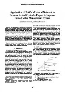
and biological data, the data were interpolated to create consistent daily values as required for the model development. The concentrations of Nostocales spp. from August 1980 to May 1992 are depicted in Figure 1. The characteristics of the measured variables are listed in Table 1. What is nonstationarity?
A time series is stationary if its statistical properties (for example, the mean and the variance) are essentially constant through time [12]. If n values z1, z2, ……, zn of
a time series were observed, a plot of these values (against time) can be used to help to determine whether a time series is stationary. If the n values seem to fluctuate with constant variation around a constant mean, then it is reasonable to believe that the time series is stationary. If the n values do not fluctuate around a constant mean or do not fluctuate with constant variation, then it is reasonable to believe that the time series is nonstationary. The population behaviors of Nostocales spp. in the River Darling show nonstationarity
TABLE 1 - Characteristics of the measured variables in the River Darling from August 1980 to May 1992. Variable Temperature (℃) Turbidity (NTU) Electrical conductivity (µs/cm) pH Color (HU) Silica (µg/L) Total kjeldahl nitrogen (mg/L) Soluble reactive phosphorus (mg/L) Flow (ML/day) Nostocales spp. (cells/L)
Mean
Standard Deviation
Min
Max
18.528 117.72 496.92 7.9289 23.027 16.174 0.93297 0.1528 4211.2 18755
5.3868 89.842 200.87 0.37703 30.106 7.6821 0.34096 0.10487 5981 83653
7.5 10 175 7.1 2 0.5 0.1 0.01 65 0
29.5 500 1150 8.8 245 66.9 3.36 0.96 22056 9.2189e+005
The daily populations of Nostocales spp. in the River Darling from 1981 to 1991 constitute a time series which describes the population behaviors of Nostocales spp. (Fig. 1). The populations of Nostocales spp. apparently do not fluctuate around a constant mean and do not fluctuate with constant variation. Furthermore, the yearly means and standard deviations (Table 2) vary with great magnitude. Therefore, the population behaviors of Nostocales spp. in the River Darling show nonstationary.
TABLE 2 - Yearly means and standard deviations of Nostocales spp. populations in the River Darling from 1981 to 1991. Year 1981 1982 1983 1984 1985 1986 1987 1988 1989 1990 1991
Mean (cells/L) 2500.7 2457.4 433.78 176.34 58720 38119 91142 12506 13.5 3877 1990
Standard Deviation (cells/L) 4966.4 6415.2 927.56 530.71 1.7457e+005 53001 1.9208e+005 30753 190.71 15321 7145.1
Moreover, we think that algal population behaviors in other aquatic ecosystems are more likely to be nonstationary, instead of stationary; and some other behaviors in ecosystems also are more likely to show nonstationarity.
FIGURE 1 - The concentration of Nostocales spp. in the River Darling from July 1981 to July 1991.
Why ecosystems may be particularly susceptible to nonstationarity? Quite often, there are some changes in the underlying factors (monitored or not) influencing an ecosystem. Sometimes they change slowly, e.g environmental deterioration or environmental recovering processes. But sometimes something drastic (system shock) happens and this induces a radical change in the ecosystem. Abnormal climates or severe pollution events lead to sudden shocks to the ecosystem. Changes to the underlying factors (temperature, humidity, pH, nutrition, etc.) influencing the ecosystem lead to behavioral pattern changes. Accordingly, the behaviors of the ecosystem show nonstationarity.
305
© by PSP Volume 16 – No 3. 2007
Fresenius Environmental Bulletin
Nonstationarity was not considered seriously in previous researches on algal population behaviors, because it cannot reflect the underlying factors in change, a nonadaptive model is likely to forecast nonstationary systems with worse and worse performance when the time elapses. To forecast the future behaviors of a nonstationary system, the forecast model needs to adapt to changing underlying factors influencing the system. While many researchers [5-11] recommended neural network based models to predict phytoplankton population behaviors, none of them had adaptive ability to deal with the nonstationarity of phytoplankton population behaviors. All those models were trained once, and then used to predict algal populations without any changes when the time passed. They were assumed to accommodate all changes in aquatic systems. Nevertheless, that is impossible in the real world because no one can say with confidence that a complex aquatic ecosystem has shown all its feasible behaviors in the past. Furthermore, some models forecasted phytoplankton populations using both past and future information. For examples, Jeong et al. [9] utilized the historical information of environmental factors from 1995 to 1998 to train a neural network model in order to predict the algal populations of 1994 in the Nakdong River, Korea; Recknagel et al. [13] forecasted the phytoplankton populations in 1986 using the limnological information from 1984 to 1985 and from 1987 to 1993 in Lake Kasumigaura, Japan, and forecasted the phytoplankton populations in 1997 using the limnological information from 1988 to 1996 and 1998 to 2000 in Lake Soyang, Korea. However, future information could not be obtained to train models to forecast future behaviors. How can a forecasting model accommodate the changes to the underlying factors driving a system? Only an adaptive model can do it. A common solution for this problem is to re-estimate the model parameters using the most recent information about the system. To deal with changes of underlying factors, the moving window technique is often incorporated into forecasting models to provide adaptive ability. The moving window technique
The performance of a forecasting model depends on the training method, and upon which dataset it is trained. The training is a process by which the model parameters are estimated. The moving window approach is one method for organizing a data set for the training process. The moving window technique assumes that only near past data contains valuable information for the current prediction. Therefore, the forecasting model needs to be trained using a near past data set for a specific prediction. The near past is determined by the size of the moving window. When using the moving window, data beyond a certain age is eliminated from the training set. For example, if the window size is 2 years, the training data set contains only data with the age of less than or equal to 2 years.
The proper size of moving window depends upon the data set. Removing too much data can ignore important information, and keeping too much can include a rule that no longer applies, or is less influential [14]. So finding the proper window size is often a critical balance, and is presently more of an art than a science. A common approach is to vary the window size and measure the error. The window size with the best forecasting performance is selected. This is a trial and error approach, but can indeed be successful. Radial basis function (RBF) neural networks
A RBF neural network is a type of feedforward neural network that learns using a supervised training technique. The response of a RBF decreases or increases, monotonically with the distance from its center point [15, 16]. RBF networks are able to approximate any reasonable continuous function mapping with a satisfactory level of accuracy [15, 17]. A RBF neural network is usually comprised of three different layers - an input layer, a hidden layer, and an output layer. The input vectors are applied to all neurons in the hidden layer, which in turn are connected directly to all elements in the output layer. Detailed descriptions of the RBF network have been presented by Moody and Darken [18] and Haykin [19]. A node in the hidden layer will produce a greater output when the input vector presented is close to its center. The output of such a node will decrease as the distance from the center increases, assuming that a symmetrical basis function is used. Thus, for a given input vector, only the neurons whose centers are close to the input pattern will produce nonzero activation values to the input stimulus. The network output is formed by a linearly weighted sum of the outputs of RBF nodes in the hidden layer. The hidden layer performs a fixed nonlinear transformation with no adjustable parameters and it maps the input space into a new space. The output layer then implements a linear combiner on this new space, and the only adjustable parameters are the weights of this linear combiner. Training an RBF network involves determining the number of RBF nodes, the corresponding centers and the width of RBFs, and the output layer weight matrix. There are various ways to train the RBF network, which vary from random selection to the use of mathematical algorithms such as the genetic algorithm [20] or the orthogonal least squares learning algorithm [21]. In our study, the orthogonal least squares learning algorithm was selected for the network training. According to this algorithm, the number of hidden neurons at the beginning of training is zero. The hidden neurons are added one by one into the hidden layer until the output of the network is within a target precision. For every iteration, the sum squared error from the network is computed. If the error is lower than the pre-defined error goal, the training is stopped. If the sum squared error is above the error goal the input pattern with the largest error is identified and added to the hidden layer, which results in the maximum lowering of the net-
306
© by PSP Volume 16 – No 3. 2007
Fresenius Environmental Bulletin
work error. This process is repeated until the error value falls below the error goal [22]. The adjustment of the connection weight between the hidden layer and the output layer is performed with a least-squares solution after the selection of centers and the width of RBFs. The solution computed by the RBF network is optimal from the viewpoint of approximation theory [23]. Optimality here means that the network minimizes a function that measures how much the solution deviates from its true value as represented by the training data. Given the training data, more important, the solution for the training process is fully defined by the width of RBFs and the error goal when using orthogonal least squares learning algorithm. Therefore, the RBF network is selected in this study. The model implementation
In this study, the RBF neural network was selected as the forecaster. Instead of being trained only one time for all the predictions, the RBF neural network needs to be trained one time for any specific prediction using the training data set chosen by the moving window. Therefore, the time window of the training data set slid forward when the time of the specific prediction moved forward. To implement the model, the structure of inputs and outputs need to be determined first. Water temperature, pH, flow, color, turbidity, electrical conductivity, total Kjeldahl nitrogen, soluble reactive phosphorus and silica were selected as the input variables in our study. Maier and Dandy [24] stated that input lags have important influence on the performance of neural networks. In this study, we tried different input lags for a better performance. Finally, we chose 1, 5, 10 days lagged inputs for all the input variables to forecast the 3-days-ahead populations of Nostocales spp. Because of the magnitude difference of different variables, the training data were normalized before the model training and the outputs of the model were unnormalized for the actual predictions of the phytoplankton populations. Given the specified structure of the input-output, the moving window incorporated RBF neural network model is fully defined by the size of the moving window, the width of RBFs, and the error goal for the training. In this study three choices were tried for the size of the moving window (540 days, 900 days and 1260 days), four choices for the width of RBFs (5, 8, 11, 14) and 10 choices for the sum squared error goal (10 choices - 15, 20, …, 60 for the window size of 540 days; 10 choices - 20, 30, …, 110 - for the window size of 900 days; 10 choices - 30, 45,…, 165 - for the window size of 1260 days). In sum, 120 model parameter combinations of different window size, different widths of RBFs, and different error goals were tried. In the experiments, the forecasting performance of the models with different parameter combinations was evaluated by the correlation coefficient (R2) of the predicted and
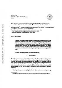
observed phytoplankton populations. Finally, three RBFNN models with best performance were identified for the window size of 540 days, 900 days, and 1260 days respectively. The neural network toolbox of Matlab 7.0 was used for the implementation of all models in this study. RESULTS AND DISCUSSION The three RBF neural network models with best performance have parameter combinations of {540 days, 25, 8}, {900 days, 40, 8}, {1260 days, 75, 5} as their window size, error goal, RBF width respectively and the correlation coefficients between their predictions and observed populations were 0.960, 0.950, 0.932 respectively. Panel A of the Figure 2 presents the predictions of the 540 days model from March 1985 to May 1992; the predictions of the 900 days model and the 1260 model are plotted in panel B and panel C. As shown in Figure 2, the three RBF neural network models could predict the timing and magnitude of major blooms of Nostocales spp. in the River Darling while they missed some algal population peaks, overestimated some peaks, and even generated some peaks that did not existed. The 540 days model and 900 days model made more overestimations after the major blooms in 1987 and 1988 than the 1260 days model, and they missed the moderate or small population peaks in 1990 and 1991. The model with a smaller window size would discard more distant past information. Because of this, such models would be more likely to produce overestimations or non-existing peaks after severe blooms and to miss moderate or small blooms after long non-bloom periods. Also because of this, such models could adapt to changed behavior patterns of algal population more quickly. For example, the 540 days models identified the second moderate peaks of algal population in 1985 while the other two models missed. In sum, the window size has a critical influence on the performance of moving window incorporated RBF neural network models. While models with smaller window size will adapt the changes of underlying factors more quickly, they can not reflect the behavior patterns of the long past, which may still be influential. On the contrary, models with a larger window size may keep too much behavior patterns, which may no longer apply, or are less influential. To lower the influence of the window size on forecasting performance, an adaptive combiner was implemented to construct a combined forecaster based on the three trained models with different window size. The combined forecaster made every prediction based on the predictions of the three trained models aforementioned. For a specific prediction, the combined forecaster first checked the performance of the three models by measuring the mean absolute error in the last three predictions. Then the prediction of the RBFNN model with the lowest error was selected as the prediction of the combined forecaster. This procedure was repeated for the next prediction.
307
© by PSP Volume 16 – No 3. 2007
Fresenius Environmental Bulletin
FIGURE 2 - The predicted populations of Nostocales spp. in the River Darling from March 1985 to May 1992 (Panel A: the 540 days RBFNN model; Panel B: the 900 days RBFNN model; Panel C: the 1260 days RBFNN model; Panel D: the combined model).
The combined forecaster, as shown in the panel D of Figure 2, could adapt to changed behavior patterns of algal population more quickly than the 540 days models. Further, the combined model produced fewer overestimations and less non-existed peaks after severe blooms just like the 1260 days model did. Therefore, the combined forecaster possesses the virtues of all the three RBF neural network models while it does not show their disadvantages. This is also supported by the correlation coefficients between the predictions of the combined model and the observed populations, 0.965, which is a little higher than that of the other three RBFNN models. CONCLUSIONS By analyzing the historical data of Nostocales spp. in the River Darling, this paper showed that the population behavior of Nostocales spp. was nonstationary. In previous researches on the modeling and forecasting of algal
populations, nonstationarity was not considered seriously. Therefore, the moving window approach was incorporated with the RBF neural network for adaptive models which can deal with nonstationarity in this study. Through experiments, three RBF neural network models with different window size were obtained. The results revealed that they could predict the timing and magnitude of major blooms of Nostocales spp. in the River Darling, Australia, although each of them showed some advantages and disadvantages. Furthermore, an adaptive combined forecaster was implemented based on the three models, which showed superiority over the three RBFNN models. For the modeling and forecasting of phytoplankton population, especially the forecasting, this paper recommends the combined RBF neural network model incorporated with the moving window approach. Moreover, similar models might be useful for modeling and forecasting other behaviors of some nonstationary ecosystems.
308
© by PSP Volume 16 – No 3. 2007
Fresenius Environmental Bulletin
ACKNOWLEDGEMENTS This research was supported by the National Natural Science Foundation of China (No. 50209003), the National Basic Research Program of China 2002CB412300, and the Chinese Academy of Sciences Project (KSCX2-1-10).
REFERENCES [1]
[2]
[3]
[4]
Okada, M. and Aiba, S. (1983). Simulation of water blooms in a eutrophic lake: modeling the vertical migration in a population of Microsystis aeruginosa. Water Research, 20, 485-490. Reynolds, C.S. (1984). The ecology of freshwater phytoplankton, Cambridge University Press, Cambridge. Sommer, U., Gliwica, Z.M., Lampert, W. and Duncan, A. (1986). The PEG-model of seasonal succession of planktonic events in fresh waters. Arch. Hydrobiol., 106, 443-471. Kromkamp, J. and Walsby, A.E. (1990). A computer model of buoyancy and vertical migration in cyanobacteria. J. Plankton Res., 12, 161-183.
[5]
Yabunaka, K., Hosomi, M. and Murakami, A. (1997). Novel application of a back-propagation artificial neural network model formulated to predict algal bloom. Wat. Sci. Tech., 36, 89-97.
[6]
Maier, H.R. and Dandy, G.C. (1997). Modelling cyanobacteria (blue-green algae) in the River Murray using artificial neural networks. Mathematics and Computers in Simulation, 43, 377-386.
[7]
Friedrich, R. (1997). ANNA – artificial neural network model for predicting species abundance and succession of blue-green algae. Hydrobiologia, 349, 47-57.
[8]
[9]
Jeong, K.S., Recknagel, F. and Joo, G.J. (2005). Prediction and elucidation of population dynamics of the blue-green algae Microcystis aeruginosa and the diatom Stephanodiscus hantzschii in the Nakdong River-Reservior systems (South Korea) by a recurrent artificial neural network. In: Recknagel F. (Ed.) Ecological Informatics, 2nd Ed., Springer-Verlag, New York, 255-273. Jeong, K.S., Joo, G.J., Kim, H.W., Ha, K. and Recknagel, F. (2001). Prediction and elucidation of phytoplankton dynamics in the Nakdong River (Korea) by means of a recurrent neural network. Ecological Modelling, 146, 115-129.
[10] Walter, M., Recknagel, F., Carpenter, C. and Bormans, M. (2001). Predicting eutrophication effects in the Burrenjuck Reservoir (Australia) by means of the deterministic model SALMO and the recurrent neural network model ANNA. Ecological Modelling, 146, 97-113. [11] Wei, B., Sugiura, N. and Maekawa, T. (2001). Use of artificial neural network in the prediction of algal blooms. Water Resource, 35, 2022–2028. [12] Bowerman, B.L. and Connell, R. (2003). Forecasting and Time Series, third ed., Publisher: China Machine Press, Peking.
309
[13] Friedrich, R., Welk, A., Kim, B. and Takamura, N. (2005). Artificial neural network approach to unravel and forecast algal population dynamics of two lakes different in morphometry and eutrophication. In: Recknagel, F. (Ed.) Ecological Informatics, 2nd Ed., Springer-Verlag, New York, 325-345. [14] Morantz, B.H. (2002). Weighted window method for time series forecasting with an artificial neural network, Ph.D. Dissertation, Robinson College of Business, Georgia State University. [15] Park, J. and Sandberg, I.W. (1991). Universal approximation using radial basis functions network. Neural Computing, 3, 246–257. [16] Bianchini, M., Frasconi, P. and Gori, M. (1995). Learning without local minima in radial basis function networks. IEEE Trans. Neural Networks, 6, 749–756. [17] Broomhead, D.S. and Lowe, D. (1988). Multi-variable functional interpolation and adaptive networks. Complex Syst., 2, 321–355. [18] Moody, J. and Darken, C. (1989). Faster learning in networks of locally tuned processing units. Neural Computing, 1, 281294. [19] Haykin S. (1999). Neural networks: a comprehensive foundation, 2nd ed., Prentice Hall, New Jersey. [20] Sheta, A.F. and Jong, K. (2001). Time-series forecasting using GA-tuned radial basis functions. Information Sciences, 133, 221–228. [21] Chen S., Cowan, C.F.N. and Grant, P.M. (1991). Orthogonal least squares learning algorithm for radial basis function networks. IEEE Trans. Neural Networks, 2, 302-309. [22] Demuth, H. and Beale, M. (1996). Neural Network Toolbox: User’s Guide. The Math Works Inc., Natick, MA, [23] Poggio, T. and Girosi, F. (1990). Networks for approximation and learning. Proceeding of IEEE 78, 1481-1497. [24] Maier H.R. and Dandy, G.C. (2001). Neural network based modeling of environmental variables: a system approach. Mathematical and Computer Modeling, 33, 669-682.
Received: August 28, 2006 Accepted: September 29, 2006
CORRESPONDING AUTHOR Lirong Song Institute of Hydrobiology Chinese Academy of Sciences Wuhan 430072 P.R. China E-mail:
[email protected] FEB/ Vol 16/ No 3/ 2007 – pages 304 – 309