Using the SALI Method to Distinguish Chaotic and Regular Orbits in ...

Issue 3 (July)

PROGRESS IN PHYSICS

Volume 13 (2017)

Using the SALI Method to Distinguish Chaotic and Regular Orbits in Barred Galaxies with the LP-VIcode Program Lucas Antonio Carit´a1,2,3, Irapuan Rodrigues2, Ivˆanio Puerari3 and Luiz Eduardo Camargo Aranha Schiavo2 1 Instituto

Federal de Educac¸a˜ o, Ciˆencia e Tecnologia de S˜ao Paulo, IFSP, S˜ao Jos´e dos Campos, Brasil. 2 Universidade do Vale do Para´ıba, UNIVAP, S˜ ao Jos´e dos Campos, Brasil. 3 Instituto Nacional de Astrof´ısica, Optica ´ y Electr´onica, INAOE, Puebla, M´exico.

The Smaller Alignment Index (SALI) is a new mathematical tool for chaos detection in the phase space of Hamiltonian Dynamical Systems. With temporal behavior very specific to movements ordered or chaotic, the SALI method is very efficient in distinguishing between chaotic and regular movements. In this work, this method will be applied in the study of stellar orbits immersed in a gravitational potential of barred galaxies, once the motion of a test particle, in a rotating barred galaxy model is given by a Hamiltonian function. Using an analytical potential representative of a galaxy with bar (two degrees of freedom), we integrate some orbits and apply SALI in order to verify their stabilities. In this paper, we will discuss a few cases illustrating the trajectories of chaotic and regular orbits accompanied by the graph containing the behavior of SALI. All calculations and integrations were performed with the LP-VIcode program.

1 Introduction One of the schemes more used to classify galaxies according to their morphology was proposed by Edwin Powell Hubble. Basically, the Hubble fork separates galaxies in two types: regular spirals (S) and barred spirals (SB). The galaxy bar, spiral arms and even galactic rings are structures that can be interpreted as disturbance to axisymmetric potential of the galactic disk. In this work, we study the nature of some orbits immersed in analytical potentials with two degrees of freedom representing barred galaxies. In order to do this, we applied the Smaller Alignment Index (SALI) [9–13], which is a mathematical tool for distinguishing regular and chaotic motions in the phase space of Hamiltonian Dynamical Systems in analytical gravitational potentials. It is possible because the motion of a test particle in a rotating barred galaxy model is given by a Hamiltonian function. The orbits integration and the SALI calculation were performed using the LP-VIcode program [2]. The LP-VIcode is a fully operational code in Fortran 77 that calculates efficiently 10 chaos indicators for dynamic systems, regardless of the number of dimensions, where SALI is one of them. To construct our barred galaxies models, two different sets of parameters were extracted from the paper of Manos and Athanassoula [5]. The main purpose of this paper is to show some regular and chaotic orbits, where the stability study was done using the SALI method. Such orbits were taken immersed in a mathematical model for the gravitational potential that simulates a barred galaxy in a system with two degrees of freedom. 2 Methodology 2.1 The SALI method Considering a Hamiltonian flow (N degrees of freedom), an

orbit in the 2N-dimensional phase space with initial condition P(0) = (x1 (0), · · · , x2N (0)) and two different initial deviation vectors from the initial point P(0), w1 (t) and w2 (t), we define the Smaller Alignment Index (SALI) by:  SALI(t) = min kb w1 (t) + b w2 (t)k, kb w1 (t) − b w2 (t)k

(1)

where b wi (t) = wi (t)/kwi (t)k for i ∈ {1, 2}. In the case of chaotic orbits, SALI(t) falls exponentially to zero as follows: SALI(t) ∝ e−(L1 −L2 )t

(2)

where L1 and L2 are the biggest Lyapunov Exponents. When the behavior is ordered, SALI oscillates in non-zero values, that is: SALI(t) ≈ constant > 0, t −→ ∞ .

(3)

Therefore, there is a clear distinction between orderly and chaotic behavior using this method. 2.2

Gravitational potential of a barred galaxy

We apply the SALI method in the study of stellar orbits immersed in a gravitational potential of barred galaxies, once the movement of a test particle in a rotating three-dimensional model of a barred galaxy is given by the Hamiltonian: H(x, y, z, p x , py , pz ) =   = p2x + p2y + p2z + ΦT (x, y, z) + Ωb (xpy − yp x )

(4)

where the bar rotates around z; x and y contain respectively the major and minor axes of the galactic bar, ΦT is the gravitational potential (which will be described later), and Ωb represents the standard angular velocity of the bar.

Carit´a et al. Using SALI to distinguish chaotic and regular orbits in barred galaxies with the LP-VIcode

161

Volume 13 (2017)

PROGRESS IN PHYSICS

Issue 3 (July)

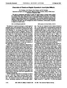
(a)

Initial Condition: (0,0.5436,0.1411,0) - Model S

(b)

Initial Condition: (0,0.1912,-0.1550,0) - Model S

(c)

Initial Condition: (0,4.2280,-0.1491,0) - Model S

(d)

Initial Condition: (0,0.9090,-0.4139,0) - Model B

(e)

Initial Condition: (0,5.7570,-0.2926,0) - Model B

(f)

Initial Condition: (0,0.4242,0.0602,0) - Model B

Fig. 1: Six orbits, each one with its SALI diagram. All orbits were integrated up to 10,000 Myr. Only the first 500 Myr were plotted in (a), (b), (d) and (f), for clarity.

For this Hamiltonian, the corresponding equations of mo- where A and B are respectively the radial and vertical scale tion and the corresponding variational equations that govern lengths, and MD is the disk mass. We represent the bar by the Ferrers Model [3]. In this the evolution of a deviation vector can be found in [4]. With such equations it is possible to follow the temporal evolution model, the density in given by  of a moving particle immersed in the potential ΦT , as well as 2    ρB (x, y, z) = ρc 1 − m2 , m < 1  verify if this orbit is chaotic or regular, following the evolu  (8)  tion of deviation vectors by the SALI method.     ρB (x, y, z) = 0 , m ≥ 1 In this work, the total potential ΦT is composed by three components, representing the galactic bulge, disk and bar: where the central density is ΦT = ΦBulge + ΦDisk + ΦBar .

(5)

We represent the bulge by the Plummer Model [8] ΦBulge = − q

GMS

,

(6)

x2 + y2 + z2 + S2

162

GMD x2 + y2 + (A +

√

(7) z2 + B2 )2

105 GMB , 32π abc

MB is the bar mass and

where S is the length scale and MS is the bulge mass. We represent the disk by the Miyamoto-Nagai Model [6] ΦDisk = − q

ρc =

x2 y2 z2 + + , a2 b2 c2 where a > b > c > 0 are the semi-axes of the ellipsoid which represents the bar. The potential created by the galactic bar is calculated with the Poisson equation (see [1]): Z 3 ρc ∞ du  1 − m2 (u) (9) ΦBar = −π G abc 3 λ ∆(u) m2 =

Carit´a et al. Using SALI to distinguish chaotic and regular orbits in barred galaxies with the LP-VIcode

Issue 3 (July)

PROGRESS IN PHYSICS

Volume 13 (2017)

(a)

Initial Condition: (0,0.0640,0.7960,0) - Model S

(b)

Initial Condition: (0,1.9932,0.0576,0) - Model S

(c)

Initial Condition: (0,3.5032,-0.2931,0) - Model S

(d)

Initial Condition: (0,2.6664,-0.2257,0) - Model B

(e)

Initial Condition: (0,3.5148,-0.0508,0) - Model B

(f)

Initial Condition: (0,5.5146,-0.2951,0) - Model B

Fig. 2: The SALI graphics has both axes in logarithmic scale. All orbits were integrated into 10,000 Myr. Only the first 5,000 Myr were plotted in (b), for clarity.

In this context, considering Ωb the bar angular velocity, our reference frame should also rotate with angular velocity Ωb . This affects the motion and variational equations since, as can be seen in [4], they depend on Ωb . In order to solve 2 2 2 2 ∆ (u) = (a + u)(b + u)(c + u) this problem, adjustments were made to the main program to and λ is the positive solution of m2 (λ) = 1 for the region include the rotation in the coordinate system with the same outside the bar (m ≥ 1) and λ = 0 for the region inside the bar angular velocity of the bar. (m < 1). 2.4 Parameters sets 2.3 The LP-VIcode program with minor adjustments We used the two parameter sets shown in Table 1 for the poTo perform the orbits integrations and the SALI calculation, tential model, taken from the paper by Manos & Athanaswe used the LP-VIcode program [2], which is an operational soula [5]. The model units adopted are: 1 kpc for length, code in Fortran 77 that calculates efficiently 10 chaos indica- 103 km s−1 for velocity, 103 km s−1 kpc−1 for angular velocity, tors for dynamical systems, including SALI. 1 Myr for time, and 2 × 1011 M solar for mass. The universal In this program, the user must provide the expressions gravitational constant G will always be considered 1 and the of the potential as well the expressions of motion and vari- total mass G(MS + MD + MB ) will be always equal to 1. ational equations. However, the general structure of motion and variational equations previously written in the main pro2.5 Initial conditions gram, take into account only a static reference frame, and it is known that in order to model the galactic bar potential, it is We emphasize that in this paper we study orbits with two denecessary to consider a coordinate system that rotates along grees of freedom. In order to do that, we consider z = 0 and pz = 0 in the three-dimensional Hamiltonian (4). with the bar.

where

y2 z2 x2 + 2 + 2 , m (u) = 2 a +u b +u c +u 2

Carit´a et al. Using SALI to distinguish chaotic and regular orbits in barred galaxies with the LP-VIcode

163

Volume 13 (2017)

PROGRESS IN PHYSICS

Issue 3 (July)

Table 1: Parameter Sets and the Bars Co-rotation.

Model S Model B

MS 0.08 0.08

S 0.4 0.4

MD 0.82 0.82

A 3.0 3.0

B 1.0 1.0

MB 0.1 0.1

a 6.0 6.0

b 1.5 3.0

c 0.6 0.6

Ωb 0.054 0.054

CR 6.04 6.06

The effective potential, which is the sum of the gravita- 3.2 Chaotic orbits tional potential with the potential generated by the repulsive Fig. 2 shows a sample of 6 chaotic orbits, identified by their centrifugal force, is given by: SALI indexes that goes to zero after some time, as discussed in section 2.1. 1 (10) Φe f f (x) = ΦT (x) − |Ω × x|2 . 2 4 Conclusion Written like that, this potential represents a rotating system. In this study, we were able to reproduce a mathematical modThe quantity eling of the gravitational potential of a barred galaxy and, in 1 E J = |v|2 + Φe f f (x) (11) order to verify the stability of the orbits within, we applied the 2 SALI method. We were able to prove the SALI efficiency in is called Jacobi Energy and is conserved in the rotating sys- distinguishing regular or chaotic orbits. In fact, this method tem. offers an easily observable distinction between chaotic and The curve given by Φe f f (0, y, 0) = E J is called Zero Ve- regular behavior. locity Curve and provides a good demarcation for the choice We also perceive the LP-VIcode efficiency, which proved of initial conditions, since there is only possibility of orbits to be extremely competent in the orbits integration and study when Φe f f ≤ E J , in other words, below this curve (see [1]). of stability with SALI. To make an adjustment in the variaTherefore, we generated some random initial conditions tional and motion equations programmed in the LP-VIcode, initially taking a value to y0 less than the highest possible we insert an adaptation in the main code to take into account value of y for a given energy E J , taking x0 = 0 and vy0 = 0. a rotating system. This done, we could calculate v x as follows: Therefore, we conclude that we were successful in calculating these orbits and confirm the SALI method as a new   1 1 2 EJ = v x0 + v2y0 + Φe f f = v2x0 + Φe f f (12) important tool in the study of stellar orbits stability. 2 2 and this implies Acknowledgements q We acknowledge the Brazilian agencies FAPESP, CAPES and (13) v x0 = ± 2(E J − Φe f f ) . CNPq (200906-2015-1), as well as the Mexican agency COThen we constructed initial conditions (x0 , y0 , v x0 , vy0 ) to NACyT (CB-2014-240426) for supporting this work. Our integrate the orbits. As x0 = 0 and vy0 = 0, the launched sincere thanks to Dr. Pfenniger, who kindly provided us with orbits will always be initially over the y axis and will have his Fortran 77 implementation of the Ferrers bar potential. All the numerical work was developed using the Hipercubo Clusinitial velocity only in the x direction. Notice that we have two possible velocities from equation ter resources (FINEP 01.10.0661-00, FAPESP 2011/13250-0 (13): one negative and one positive. We decided to take y0 and FAPESP 2013/17247-9) at IP&D–UNIVAP. always positive, so that when v x0 is positive, the orbits are Received on May 12, 2017 prograde (orbits that rotate in the same direction of the bar) and when v x0 is negative, the orbits are retrograde (orbits that References rotate in the opposite direction of the bar). nd 3

1. Binney J. and Tremaine S. Galactic Dynamics, 2 versity Press, 2008.

Results

ed. Princeton Uni-

In our computational calculations, we consider SALI < 10−8 close enough to zero to consider the movement chaotic.

2. Carpintero D. D., Maffione N. and Darriba L. LP-VIcode: a program to compute a suite of variational chaos indicators. Astronomy and Computing, 2014, v. 5, 19–27. DOI: 10.1016/j.ascom.2014.04.001.

3.1

3. Ferrers N. M. On the potential of ellipsoids, ellipsoidal shells, elliptic laminae and elliptic rings, of variables densities. Quarterly Journal of Pure and Applied Mathematics, 1877, v. 14, 1–22.

Regular orbits

In Fig. 1 we show 6 different orbits, each one with its SALI diagram, from where we can identify them as regular orbits, as explained in section 2.1. 164

4. Manos T. A Study of Hamiltonian Dynamics with Applications to Models of Barred Galaxies. PhD Thesis in Mathematics, Universit´e de Provence and University of Patras, 2008.

Carit´a et al. Using SALI to distinguish chaotic and regular orbits in barred galaxies with the LP-VIcode

Issue 3 (July)

PROGRESS IN PHYSICS

5. Manos T. and Athanassoula E. Regular and chaotic orbits in barred galaxies – I. Applying the SALI/GALI method to explore their distribution in several models. Monthly Notices of the Royal Astronomical Society, 2011, v. 415, 629–642. DOI: 10.1111/j.1365-2966.2011.18734.x. 6. Miyamoto M. and Nagai R. Three-dimensional models for the distribution of mass in galaxies. Astronomical Society of Japan, 1975, v. 27, 533–543. 7. Pfenniger D. The 3D dynamics of barred galaxies. Astronomy and Astrophysics, 1984, v. 134, 373–386. ISSN: 0004-6361. 8. Plummer H. C. On the problem of distribution in globular star clusters. Notices of the Royal Astronomical Society, 1911, v. 71, 460–470. DOI: 10.1093/mnras/71.5.460. 9. Skokos Ch. Alignment indices: a new, simple method for determining the ordered or chaotic nature of orbits. Journal of Physics: Mathematical and General, 2001, v. 34, 10029–10043. DOI: 10.1088/03054470/34/47/309.

Volume 13 (2017)

10. Skokos Ch., Antonopoulos Ch., Bountis T. C. and Vrahatis M. N. Smaller alignment index (SALI): Determining the ordered or chaotic nature of orbits in conservative dynamical systems. In Gomez G., Lo M. W., Masdemont J. J., eds. Proceedings of the Conference Libration Point Orbits and Applications, World Scientific, 2002, 653–664. DOI: 10.1142/9789812704849 0030. 11. Skokos Ch., Antonopoulos Ch., Bountis T. C. and Vrahatis M. N. How does the Smaller Alignment Index (SALI) distinguish order from chaos? Prog. Theor. Phys. Supp., 2003, v. 150, 439–443. DOI: 10.1143/PTPS.150.439. 12. Skokos Ch., Antonopoulos Ch., Bountis T. C. and Vrahatis M. N. Detecting order and chaos in Hamiltonian systems by the SALI method. J. Phys. A, 2004, v. 37, 6269–6284. DOI: 10.1088/0305-4470/37/24/006. 13. Skokos Ch. and Bountis T. C. Complex Hamiltonian Dynamics. Springer, 2012.

Carit´a et al. Using SALI to distinguish chaotic and regular orbits in barred galaxies with the LP-VIcode

165